Fundamental Theorem of Linear Maps¶

Theorem¶

Let $V$ be a finite-dimensional vector space and let $\boldsymbol{A} \in \mathcal{L}(V,W)$ be a linear map. Then

Interpretation¶

A linear map splits the dimension of its domain into directions lost to the kernel and directions that survive in the range. The kernel collects the input vectors sent to $\boldsymbol{0}$; the dimension of the range counts the independent output directions that can actually be reached. The theorem says that these two counts always add up to $\dim V$.

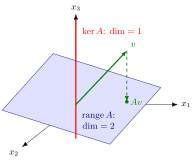
The map in the figure projects $\mathbb{R}^3$ vertically onto the shaded plane, as $\boldsymbol{v}$ drops onto $\boldsymbol{A}\boldsymbol{v}$. The whole vertical line is sent to $\boldsymbol{0}$, so $\dim(\ker \boldsymbol{A})=1$$1$, and the outputs fill the plane, so $\dim(\operatorname{range}\boldsymbol{A})=2$$2$: $1+2=3=\dim\mathbb{R}^3$$\dim {\mathbb{R}}^3$.

For an $m\times n$ matrix, read as a map $\mathbb{R}^n\to\mathbb{R}^m$${\mathbb{R}}^m$, $\dim V=n$ is the number of columns, $\dim(\operatorname{range}\boldsymbol{A})$ is the rank, the number of pivots, and $\dim(\ker \boldsymbol{A})$ is the number of free variables of the homogeneous system $\boldsymbol{A}\boldsymbol{x}=\boldsymbol{0}$$0$. The theorem is then the count "pivot columns plus free columns equals all columns".

If $\dim V=\dim W$$\dim W$, a linear map is injective if and only if it is surjective: a kernel of dimension $0$ leaves a range of full dimension. If $\dim V>\dim W$$\dim W$, the range has dimension at most $\dim W$, so the kernel is nonzero; for example, a homogeneous system with more unknowns than equations always has a nonzero solution.

A common misreading is to picture kernel and range as two pieces of $V$. The kernel lies in $V$, but the range lies in $W$; only their dimensions add up.

Key Results¶

• The theorem is also called the rank-nullity theorem: the rank of $\boldsymbol{A}$ is $\dim(\operatorname{range}\boldsymbol{A})$ and its nullity is $\dim(\ker \boldsymbol{A})$.
• It connects injectivity, surjectivity, and dimension for finite-dimensional vector spaces.

Examples¶

• If $\boldsymbol{A}\colon\mathbb{R}^3\to\mathbb{R}^2$ has a one-dimensional kernel, then its range has dimension $2$.
• If $V$ is finite-dimensional, $\boldsymbol{A}\in\mathcal{L}(V)$ and $\ker \boldsymbol{A}=\{\boldsymbol{0}\}$$\{0\}$, then $\dim(\operatorname{range}\boldsymbol{A})=\dim V$$\dim V$, so $\operatorname{range}\boldsymbol{A}=V$ and $\boldsymbol{A}$ is bijective.

Prerequisites¶

• Kernel
• Range of a Linear Map
• Dimension

Related Concepts¶

• Linear Map
• Rank

Sources¶

• Math II: Linear Algebra · Week 4

Aliases: rank-nullity theorem, dimension theorem Symbols: element of, real numbers

Last updated: 20 October 2026 03:02