Diagonalization¶

Definition¶

Diagonalization is the process of finding an invertible matrix $\boldsymbol{P}$ and a diagonal matrix $\boldsymbol{D}$ such that $\boldsymbol{A}=\boldsymbol{P}\boldsymbol{D}\boldsymbol{P}^{-1}$$\mathbf{P}\mathbf{D}{\mathbf{P}}^{-1}$, equivalently $\boldsymbol{P}^{-1}\boldsymbol{A}\boldsymbol{P}=\boldsymbol{D}$$\mathbf{D}$.

Interpretation¶

Diagonalization rewrites a linear transformation in an eigenbasis, where its action is simple coordinate-wise scaling.

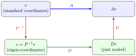
The diagram shows two routes from $\boldsymbol{v}$ to $\boldsymbol{A}\boldsymbol{v}$. The top arrow applies $\boldsymbol{A}$ directly. The detour first computes the eigen-coordinates $\boldsymbol{c}=\boldsymbol{P}^{-1}\boldsymbol{v}$${\mathbf{P}}^{-1}\mathbf{v}$, then scales each coordinate by its eigenvalue with $\boldsymbol{D}=\operatorname{diag}(\lambda_1,\ldots,\lambda_n)$$\mathrm{diag}({\lambda }_1,\dots ,{\lambda }_n)$, and finally returns to standard coordinates with $\boldsymbol{P}$. Both routes give the same vector, which is the equation $\boldsymbol{A}=\boldsymbol{P}\boldsymbol{D}\boldsymbol{P}^{-1}$ read from right to left.

In practice, find the eigenvalues as roots of the characteristic polynomial, find a basis of each kernel $\ker(\boldsymbol{A}-\lambda\boldsymbol{I})$$\lambda \mathbf{I})$, and put these eigenvectors as the columns of $\boldsymbol{P}$, with the eigenvalues in the same order on the diagonal of $\boldsymbol{D}$. This succeeds exactly when there are $n$ independent eigenvectors. The result is not unique: reordering or rescaling the eigenvectors, with the eigenvalues following, gives another valid pair.

The payoff is in powers. The inner factors cancel in $\boldsymbol{A}^k=\boldsymbol{P}\boldsymbol{D}\boldsymbol{P}^{-1}\boldsymbol{P}\boldsymbol{D}\boldsymbol{P}^{-1}\cdots$$\mathbf{P}\mathbf{D}{\mathbf{P}}^{-1}\mathbf{P}\mathbf{D}{\mathbf{P}}^{-1}\cdots$, leaving $\boldsymbol{A}^k=\boldsymbol{P}\boldsymbol{D}^k\boldsymbol{P}^{-1}$$\mathbf{P}{\mathbf{D}}^k{\mathbf{P}}^{-1}$, where $\boldsymbol{D}^k$ raises each eigenvalue to the power $k$. For $\begin{pmatrix}2&1\\1&2\end{pmatrix}$, with eigenvalues $3$ and $1$, this gives $\tfrac{1}{2}(3^k+1)$ on the diagonal of $\boldsymbol{A}^k$ and $\tfrac{1}{2}(3^k-1)$ off it. Powers of matrices return later in Math V, in linear difference systems.

A common slip is the order of the factors. With the eigenvectors as columns of $\boldsymbol{P}$, the formula is $\boldsymbol{A}=\boldsymbol{P}\boldsymbol{D}\boldsymbol{P}^{-1}$$\mathbf{P}\mathbf{D}{\mathbf{P}}^{-1}$, not $\boldsymbol{P}^{-1}\boldsymbol{D}\boldsymbol{P}$. Checking $\boldsymbol{A}\boldsymbol{P}=\boldsymbol{P}\boldsymbol{D}$ column by column, which says $\boldsymbol{A}\boldsymbol{p}_i=\lambda_i\boldsymbol{p}_i$${\lambda }_i{\mathbf{p}}_i$, settles it.

Key Results¶

• If $\boldsymbol{A}=\boldsymbol{P}\boldsymbol{D}\boldsymbol{P}^{-1}$$\mathbf{P}\mathbf{D}{\mathbf{P}}^{-1}$, then $\boldsymbol{A}^k=\boldsymbol{P}\boldsymbol{D}^k\boldsymbol{P}^{-1}$$\mathbf{P}{\mathbf{D}}^k{\mathbf{P}}^{-1}$.
• The columns of $\boldsymbol{P}$ are eigenvectors of $\boldsymbol{A}$, and the diagonal entries of $\boldsymbol{D}$ are the corresponding eigenvalues.

Examples¶

• A diagonal matrix is already diagonalized with $\boldsymbol{P}=\boldsymbol{I}$$\mathbf{I}$.
• If $\boldsymbol{A}$ has a basis of eigenvectors, then it is diagonalizable.

Prerequisites¶

• Square Matrix
• Eigenvalue and Eigenvector
• Diagonal Matrix
• Eigenbasis

Related Concepts¶

• Matrix Product
• Jordan Normal Form
• Inverse Matrix
• Diagonalizable Matrix

Sources¶

• Math II: Linear Algebra · Week 6

Aliases: diagonalisation, matrix diagonalization, eigendecomposition, eigenvalue decomposition Symbols: lambda

Last updated: 20 October 2026 03:02