Fundamental Theorem of Calculus Part 2¶

Theorem¶

Suppose $a < b$ are real numbers, and let $f\colon [a, b] \to\mathbb{R}$ be a Riemann integrable function. If $F\colon [a, b] \to\mathbb{R}$ is an antiderivative of $f\text{,}$ then

Interpretation¶

This part of the fundamental theorem turns the evaluation of a definite integral into a subtraction. Once an antiderivative $F$ of $f$ is known, the limit of Riemann sums equals $F(b)-F(a)$$F(a)$, and no sums have to be computed.

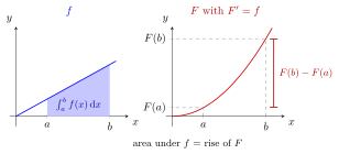
The figure uses $f(x)=x/2$ and $F(x)=x^2/4$$x^2/4$, with $a=1$ and $b=3$$3$. The area in the left panel is $2$, while the right panel rises by $F(3)-F(1)=9/4-1/4=2$$2$. The theorem equates these two quantities. Where $f$ is large, $F$ climbs steeply, and where $f$ is small, $F$ is nearly flat. This example has $f\ge0$$0$; for an integrand that changes sign, the integral measures signed area.

The reason is a telescoping sum. For a partition $P$, the mean value theorem gives points $c_i$ with $F(x_i)-F(x_{i-1})=f(c_i)(x_i-x_{i-1})$$x_{i-1})$. With these tags the Riemann sum is exactly $F(b)-F(a)$$F(a)$, for every $P$, so the integral is $F(b)-F(a)$ as well.

Both hypotheses are needed. The integral must exist: $F(x)=x^2\sin(1/x^2)$ with $F(0)=0$ is differentiable on $[0,1]$, but $F'$ is unbounded near $0$ and therefore not Riemann integrable. And $F$ must be an antiderivative on all of $[a,b]$. The function $-\arctan(1/x)$ has derivative $\frac{1}{1+x^2}$ for $x\ne0$$0$, yet its difference between $x=1$ and $x=-1$ is $-\frac{\pi}{2}$, while $\int_{-1}^{1}\frac{\mathrm{d}x}{1+x^2}=\frac{\pi}{2}$$\frac{\pi }{2}$; it jumps at $0$, so the theorem does not apply to it.

Later, the rules of integration by parts and substitution combine this theorem with the product rule and the chain rule.

Key Results¶

• Definite integrals can be evaluated using antiderivatives.
• The result depends only on boundary values.
• Integration becomes an algebraic operation once antiderivatives are known.

Examples¶

• $\displaystyle \int_0^1 x^2\,\mathrm{d}x=\frac{1}{3}\text{.}$
• $\displaystyle \int_a^b 1\,\mathrm{d}x=b-a\text{.}$

Prerequisites¶

• Definite Integral
• Antiderivative

Related Concepts¶

• Fundamental Theorem of Calculus Part 1
• Indefinite Integral

Sources¶

• Math I: Calculus · Lecture 11

Aliases: FTC 2, second fundamental theorem of calculus, Newton-Leibniz formula, Newton-Leibniz theorem Symbols: integral, pi, real numbers

Last updated: 27 October 2026 11:52