Economic Order Quantity¶

Proposition¶

Under the classical EOQ assumptions with $D,K,h>0$ $0$ , the unique order quantity minimizing the total cost per unit time (TCU) $TCU(y)=KD/y+hy/2$ over $y>0$ is

y^*=\sqrt{\frac{2KD}{h}},\qquad t_0^*=\frac{y^*}{D}=\sqrt{\frac{2K}{Dh}}.

The optimal policy orders $y^*$ units when stock reaches zero.

Interpretation¶

The economic order quantity is the batch size at which the setup cost rate $KD/y$ and the holding cost rate $hy/2$ of the classical EOQ model are in balance. Larger batches cut the number of setups; smaller batches cut the average stock.

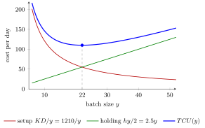
The setup cost per unit time, falling as the order size grows, the holding cost, rising linearly, and their sum, a U-shaped total cost with its minimum at the order size 22.

The setup curve $1210/y$ falls and the holding line $2.5y$ rises; they cross at $y=22$ $22$ , where each equals $55$ . The total cost is lowest exactly there, at $110$ per day.

Change $D$ , $K$ and $h$ : the minimum of $TCU(y)$ sits where the two cost rates are equal, at $y^*=\sqrt{2KD/h}$ $2 K D / h$ .

That the minimum lies at the crossing is no coincidence. The product of the two terms, $\frac{KD}{y}\cdot\frac{hy}{2}=\frac{KDh}{2}$ $\frac{K D h}{2}$ , does not depend on $y$ , and for two positive numbers $a+b\ge2\sqrt{ab}$ $2 ab$ , since $(\sqrt{a}-\sqrt{b})^2\ge0$ $0$ . Hence

TCU(y)\ge2\sqrt{\frac{KDh}{2}}=\sqrt{2KDh},

with equality if and only if $KD/y=hy/2$ $h y /2$ , that is $y^2=2KD/h$ $2 K D / h$ . This inequality gives the same answer as setting the derivative to zero.

The square root makes the answer move slowly with the data: doubling demand raises $y^*$ only by a factor $\sqrt{2}\approx1.41$ $1.41$ . The cost curve is also flat near its minimum: batches of $11$ or $44$ phones instead of $22$ cost $137.5$ per day instead of $110$ , so an order size somewhat away from $y^*$ costs little extra. The same formula reappears with lead times, is corrected by a factor with planned shortages, and serves as a candidate with price breaks.

Key Results¶

At the optimum, $KD/y^*=hy^*/2$ $h y^{*} /2$ .
The minimum relevant cost rate is $\sqrt{2KDh}$ .
Increasing demand raises the batch size but shortens the ordering cycle.
The formula follows from $-KD/y^2+h/2=0$ and strict convexity.

Examples¶

For the illustrated phone shop, $K=605$ $605$ , $D=2$ per day and $h=5$ per unit per day give $y^*=\sqrt{2\cdot605\cdot2/5}=22$ $22$ . It orders every $22/2=11$ days; setup and holding each cost $55$ per day, giving relevant daily cost $110$ .
The snack bar obtains $y^*=\sqrt{2(50)(10)/(3/7)}\approx48.30$ kilograms.

Prerequisites¶

Classical EOQ Model
Differentiation

Sources¶

OR Modelling · Week 5

Aliases: EOQ, EOQ formula, Wilson formula, Harris-Wilson formula, economic order quantity formula Symbols: square root

Last updated: 20 October 2026 03:02