Zero-Inventory Ordering Property¶

Proposition¶

In the course's uncapacitated dynamic lot-size special case, assume no shortages or lead time, nonincreasing marginal production and holding costs, and zero initial inventory. There exists an optimal policy with

y_ix_i=0\qquad(i=1,\ldots,n).

Thus a positive order is placed only when starting stock is zero, and it covers the exact demand of one or more consecutive periods.

Interpretation¶

The property says that, under its cost assumptions, there is an optimal policy in which no order is placed while stock is still on hand. Each order then covers the full demand of a run of consecutive periods, so instead of every integer order size, only the sums $D_i+\dots+D_t$ need to be considered.

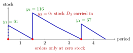
A stock level over four periods with orders of 61, 116 and 67 placed only when the stock has dropped to zero, and no order in period 3.

The first order, $61$ , is placed at zero stock and lasts exactly through period 1. The order of $116$ covers periods 2 and 3, with demands $62$ and $54$ , so period 3 orders nothing ( $y_{3} =$ $y_3=0$ $0$ ) and starts with $54$ units. The last order, $67$ , follows when stock is zero again. Every order sits at a red dot at zero stock, so $y_ix_i=0$ in every period.

The assumptions matter: when ordering costs rise faster than the quantity, splitting a quantity over two orders can be cheaper, and then an optimal policy may carry stock into a period that orders. With ordering cost $y_i^2$ and no setup cost, for instance, two orders of $2$ cost $8$ , while one order of $4$ costs $16$ .

Under the property, the lot-size recursion only needs order sizes that are sums of consecutive demands, and the Silver-Meal heuristic builds its orders the same way, without the guarantee of optimality. A common slip is to read the property as a statement about every optimal policy: it guarantees one optimal policy of this form, and tied optima may look different.

Key Results¶

The statement guarantees an optimal policy of this form; it need not describe every tied optimum.
The special case is not justified for increasing marginal ordering costs, as in the general example.
The course handles positive initial stock by subtracting it from successive demands until exhausted.

Examples¶

In the four-period example, initial stock 15 reduces first-period demand from 76 to 61.
The optimal orders $(61,116,0,67)$ cover period 1, periods 2-3, and period 4, at total cost 860.

Prerequisites¶

Silver-Meal Heuristic

Sources¶

OR Modelling · Week 6

Aliases: Zero-inventory ordering, Wagner-Whitin property, zero-inventory property

Last updated: 20 October 2026 03:02