Price-Break Indifference Quantity¶

Proposition¶

Let $y_m=\sqrt{2KD/h}$ and $TCU_j(y)=Dc_j+KD/y+hy/2$ $h y /2$ , with $c_1>c_2$ $c_{2}$ . The price-break indifference quantity $Q>y_m$ solves

TCU_2(Q)=TCU_1(y_m),

or equivalently

Q^2+\frac{2(c_2D-TCU_1(y_m))}{h}Q +\frac{2KD}{h}=0.

Interpretation¶

The indifference quantity answers how far above the EOQ a price-break threshold may lie and still be worth reaching. Up to $Q$ , the purchasing discount on every unit outweighs the extra setup and holding costs of the larger batch; beyond $Q$ it does not.

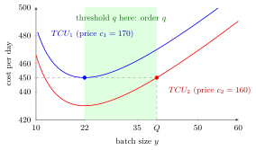
Two total-cost curves for the two unit prices, a horizontal line at the minimum 450 of the higher-price curve, and a shaded band of thresholds up to 39.86 where ordering the threshold quantity is cheaper.

The horizontal line at $450$ is the best cost without discount, $TCU_1(22)$ . The discounted curve $TCU_2$ lies below it from $22$ up to $Q\approx39.86$ $39.86$ , where it climbs back to $450$ . A threshold $q$ in the shaded band, such as $35$ , should be reached; a threshold beyond $Q$ should not.

$Q$ is where the discounted cost curve climbs back to the best cost without discount, $TCU_1(y_m)$ . Move $q$ past $y_m$ and past $Q$ to see the three cases.

At $y_m$ the discount saves $D(c_1-c_2)=2\cdot10=20$ per day. Moving the batch from $y_m$ to $Q$ raises setup and holding cost from $110$ to $130$ per day, which uses up exactly that saving. Multiplying $TCU_2(Q)=TCU_1(y_m)$ by $2Q/h$ gives the quadratic equation of the Proposition. It has two solutions, for the phones about $12.14$ and $39.86$ ; the smaller one lies below $y_m$ , and a threshold below $y_m$ needs no comparison, since $y_m$ itself then qualifies for the discount. Only the larger solution is a useful boundary.

$Q$ is not an optimal order quantity itself: it is a boundary for the threshold $q$ . In practice it is enough to compare the full costs of the two candidates $y_m$ and $q$ , as in EOQ with price breaks; $Q$ shows at once which thresholds are worth reaching.

Key Results¶

With the worked-example convention that $q$ qualifies, a threshold $y_m<q<Q$ favours ordering $q$ .
For $q>Q$ $Q$ , retain $y_m$ ; for $q<y_m$ $y_{m}$ , $y_m$ already receives the discount.
At $q=Q$ $Q$ , the two candidates tie.
Directly comparing candidate costs avoids solving for $Q$ .

Examples¶

The snack-bar exercise gives $Q\approx89.07$ kilograms; its threshold 100 is too high.
For the phone example, $Q\approx39.86$ $39.86$ , and threshold 35 lies between $y_m=22$ and $Q$ .

Prerequisites¶

EOQ with Price Breaks

Economic Order Quantity

Sources¶

OR Modelling · Week 5

Symbols: square root

Last updated: 22 October 2026 19:04