Reduced Cost¶

Definition¶

In the course's maximization sensitivity report, the reduced cost of a currently zero-valued variable is the marginal change in the objective when that variable is increased and the other variables adjust through the current basis. If the tableau row is $z+q_jx_j+\cdots=z_0$$z_0$, the corresponding reduced cost is $-q_j$.

Interpretation¶

The reduced cost of an activity that is not used at the optimum says what happens to the objective if one unit of it is forced into the plan while the other variables adjust to keep the constraints satisfied. It is the opportunity cost of that activity: a negative value means that a small forced increase reduces profit.

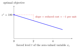
The line starts at $z^*=180$ for $t=0$ and falls by $1$ for every unit of the product $x_c$ forced into the plan, so its slope $-1$ is the reduced cost. As the Example computes, one unit of $x_c$ earns $4$ but uses hours worth $5$ at the current shadow prices.

The sign follows from the tableau. The row $z+q_jx_j+\cdots=z_0$ gives $z=z_0-q_jx_j-\cdots$$\cdots$, so raising the nonbasic variable $x_j$ by one unit changes $z$ by $-q_j$. At an optimal tableau of a maximization problem every $q_j\ge0$ by the optimality test, so the reduced costs of nonbasic variables are at most $0$ there.

In sensitivity analysis the reduced cost also says how much more profitable an unused activity would have to be: raising its coefficient by the size of the reduced cost makes it break even, so the allowable increase of a nonbasic variable equals that size, as for the sheets in the Examples. A common slip is to read the reduced cost as the profit coefficient itself; it is that coefficient minus the value of the resources the activity uses.

Key Results¶

• Do not confuse a reported reduced cost with the original objective coefficient.
• The sign is opposite to the coefficient in the course maximization tableau.
• The interpretation is local and relies on a feasible basis adjustment.

Examples¶

In the figure, a third product $x_c$ earns 4 and uses 3 finishing and 2 carpentry hours. At shadow prices 1 and 1, its reduced cost is $4-(3\cdot1+2\cdot1)=-1$$-1$. A small forced increase therefore costs 1 unit of profit per unit produced while the basis remains feasible. Raising its profit by 1 removes that marginal disadvantage; a tie need not force it into every optimal solution.

• Sheets have reported reduced cost -3.3 in the pipes-and-sheets example.
• Their profit coefficient is 4 and its allowable increase is 3.3 before the current optimal basis can cease to be optimal.

Prerequisites¶

• Simplex Tableau
• Sensitivity Analysis

Related Concepts¶

• Objective Coefficient Range
• Excel Sensitivity Report

Sources¶

• OR Modelling · Week 3

Last updated: 20 October 2026 03:02