Newsvendor Price Sensitivity¶

Proposition¶

For a fixed integer quantity $y$ and fixed purchase cost $c$ and salvage value $s<c$ $c$ , newsvendor price sensitivity finds selling prices $p>c$ for which $y$ remains optimal. The condition is

F(y-1)\le\frac{p-c}{p-s}\le F(y).

The endpoints include ties with neighbouring quantities.

Interpretation¶

The question is how far the selling price can move before a chosen order stops being optimal. The price enters the newsvendor model only through the critical ratio $\beta=(p-c)/(p-s)$ $s)$ , so the question becomes: for which prices does $\beta$ stay between the two CDF values that make $y$ optimal?

The critical ratio as a function of the selling price, rising with the price, with a shaded range of prices from 250 to 450 over which ordering 10 stays optimal.

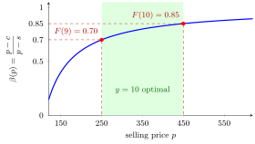
With $c=110$ and $s=50$ $50$ , the curve $\beta(p)=(p-110)/(p-50)$ rises with $p$ . It reaches $F(9)=0.70$ at $p=250$ and $F(10)=0.85$ at $p=450$ $450$ , so $y=10$ is optimal for every price in the shaded interval $[250,450]$ . Below $250$ the target probability drops under $0.70$ and fewer units are optimal; above $450$ it exceeds $0.85$ and more units are optimal.

Fix the quantity $y$ and vary the price $p$ : $y$ stays optimal while $F(y-1)\le\frac{p-c}{p-s}\le F(y)$ $F (y)$ .

The two inequalities come from the discrete newsvendor rule. The condition $\beta\le F(y)$ says that adding unit $y+1$ does not lower the expected cost, and $F(y-1)\le\beta$ says that removing unit $y$ does not lower it. At an endpoint one of them holds with equality and a neighbouring quantity is equally good. Since $\beta=1-(c-s)/(p-s)$ increases with $p$ , the set of prices is an interval, and solving $\beta(p)=F$ gives each endpoint:

p=\frac{c-Fs}{1-F}.

So the optimal quantity, as a function of the price, is constant on intervals and jumps at their endpoints. This is the newsvendor version of sensitivity analysis for linear programs, where a coefficient may move within a range without changing the optimal solution.

Key Results¶

The condition is for being an optimum, not necessarily the smallest optimum.
At the lower boundary, $y-1$ can tie with $y$ .
This analysis holds the demand distribution fixed, as the exercise does.

Examples¶

At $p=250$ $250$ , quantities 9 and 10 tie; at $p=450$ $450$ , quantities 10 and 11 tie. Increasing price past the upper endpoint calls for additional stock, with demand distribution held fixed.

The dress solution uses effective unit cost $c=80+30=110$ and salvage $s=50$ $50$ .
For $y=10$ $10$ , $F(9)=0.70$ and $F(10)=0.85$ give $250\le p\le450$ $450$ .

Prerequisites¶

Discrete Newsvendor Rule

Sources¶

OR Modelling · Week 6

Symbols: beta

Last updated: 20 October 2026 03:02