EOQ with Lead Times¶

Definition¶

The EOQ model with lead times retains constant known demand, no shortages, and the classical setup and holding costs, but an order arrives after a fixed delay $L\ge0$ $0$ . The optimal quantity remains $y^*=\sqrt{2KD/h}$ $2 K D / h$ . In the course's repeating on-hand-stock convention, order when stock falls to $DL_e$ , where $L_e$ is the effective lead time.

Interpretation¶

A lead time is the delay between placing an order and receiving it. With constant known demand, a delay only shifts the moment of ordering: the order is placed early enough that the batch arrives exactly when stock runs out, and the batch size stays the EOQ.

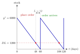
A sawtooth stock level with a horizontal reorder level at 1200; an order is placed when the stock reaches this level and arrives 12 days later, just as the stock runs out.

Stock falls from $y^*=6000$ at $100$ per day. The order is placed on day $48$ , when stock reaches the reorder level $DL=1200$ $1200$ , and arrives on day $60$ , just as stock hits zero. The remaining $1200$ pencils are exactly the demand during the $12$ -day delay.

Change the lead time $L$ : the batch size stays $y^*$ , but the order must be placed when stock reaches $DL_e$ (dashed).

The stock pattern over time is the same sawtooth as in the classical EOQ model; only the ordering moments have moved. Setup and holding costs per unit time are therefore unchanged, and so are $y^*$ and the minimum cost. The trigger has become a stock level instead of the moment stock reaches zero.

The rule $DL$ assumes that the delay is shorter than an ordering cycle. For longer delays, $DL$ exceeds $y^*$ , a level that on-hand stock never reaches from below. The effective lead time then removes the full cycles and gives the level $DL_e$ . The reasoning also relies on demand and delay being known exactly: if either were uncertain, stock could run out before the order arrives.

Key Results¶

If $L<t_0^*$ $t_{0}^{*}$ , the reorder stock level is $DL$ .
If lead time exceeds an ordering cycle, several orders can be outstanding; use the course effective-lead-time construction.
The on-hand trigger describes steady-state cycles, not the initial setup of an empty supply pipeline.

Examples¶

For the illustrated pencil inventory, demand is $D=100$ per day, each order costs $K=180$ $180$ , and holding one pencil costs $h=0.001$ per day. The optimal order quantity and relevant daily cost are

y^*=\sqrt{\frac{2KD}{h}}=\sqrt{\frac{2\cdot180\cdot100}{0.001}} =6000,\qquad \sqrt{2KDh}=6.

The cycle lasts $t_0^*=y^*/D=60$ days. With a 12-day lead time, the reorder level is $DL=1200$ $1200$ : place the order on day 48 so that it arrives on day 60, when the stock runs out. The order quantity and cost remain unchanged.

Prerequisites¶

Inventory Policy

Sources¶

OR Modelling · Week 5

Aliases: EOQ with positive lead time Symbols: square root

Last updated: 22 October 2026 19:04