Production-Inventory Model¶

Definition¶

A production-inventory model chooses production $P_t$ and end-of-period stock $I_t$ to meet known demands $d_t$ across periods. With given initial stock $I_0$ , unit production costs $c_t$ , and end-of-period holding costs $h_t$ , the course problem is represented by

\min\sum_{t=1}^T(c_tP_t+h_tI_t),\qquad I_{t-1}+P_t-d_t=I_t,\qquad P_t,I_t\ge0.

Interpretation¶

The model decides when to produce, not only how much. Production in a cheaper month may be stored for a later month at a holding cost, and the inventory balance ensures that every unit sold comes from current production or previously held stock.

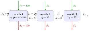
Three months in a row with production entering from above, demand leaving from below, and inventory carried from one month to the next at a holding cost.

Each month in the figure is a balance: stock arriving from the previous month plus production equals demand plus stock carried out. In month 1, $I_0=0$ and $P_1=120$ meet $d_1=100$ and leave $I_1=20$ $20$ , which is carried into month 2 at a cost of 8 per window.

The balance $I_{t-1}+P_t-d_t=I_t$ is what links the months: without it each month would be a separate problem. The nonnegativity of $I_t$ excludes shortages, so demand must be met on time. The objective then weighs producing early against producing late: a month-3 window made in month 2 costs $45+8=53$ $53$ , less than the 55 it costs in month 3, so producing early pays whenever the earlier unit cost plus the holding costs is lower, as long as capacity allows.

Linear program formulation introduces production and inventory decisions, balance equations and capacity restrictions; with continuous $P_t$ and $I_t$ the model is an LP. The same balance returns in the dynamic lot-size model, where every order also carries a fixed setup cost.

Key Results¶

Nonnegative inventory rules out shortages.
The window example charges a holding cost of 8 per window per month on end-of-month inventory.
The six-month exercise does not specify initial stock; taking $I_0=0$ is an explicit modelling assumption.
With positive production and holding costs and no required final stock, surplus final inventory is unnecessary.

Examples¶

Month 1 requires 100 windows; producing 120 from zero stock leaves 20.
Producing a month-3 window in month 2 costs 45 plus 8 holding, compared with 55 in month 3.

Prerequisites¶

Linear Program Formulation

Sources¶

OR Modelling · Week 2

Symbols: sum

Last updated: 22 October 2026 19:04