Dynamic Lot-Size Model¶

Definition¶

The dynamic lot-size model chooses order quantities over $n$ discrete periods with known varying demands, no shortages, and no lead time. In the detailed course notation, $y_i$ is the period- $i$ order, $D_i$ demand, $x_i$ starting stock, $K_i$ setup cost, $c_i(y_i)$ the variable ordering cost of $y_i$ units, and $h_i$ holding cost per unit carried to the next period. Then

\begin{gathered} x_{i+1}=x_i+y_i-D_i\ge0,\\ C_i(y_i)=\begin{cases}0,&y_i=0,\\K_i+c_i(y_i),&y_i>0.\end{cases} \end{gathered}

Minimize $\displaystyle \sum_{i=1}^n[C_i(y_i)+h_ix_{i+1}]$ $h_{i} x_{i + 1}]$ , with given $x_1$ and terminal stock $x_{n+1}=0$ in the course examples.

Interpretation¶

The dynamic lot-size model plans orders over a finite number of periods whose demands are known but differ. Each order triggers a setup cost, so it can be cheaper to order once for several periods and carry the surplus, paying holding cost for it.

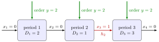
Three periods in a row with demands 2, 1 and 3, an order of 2 in each period, and the stock carried between periods, including one unit carried from period 2 into period 3.

Each box is one period with its demand, and the arrows on top are orders. The balance $x_{i+1}=x_i+y_i-D_i$ can be followed from left to right: period $1$ starts empty, orders $2$ and uses $2$ , so $x_2=0$ $0$ ; period $2$ orders $2$ but uses only $1$ , so one unit is carried into period $3$ at cost $h_2$ ; period $3$ orders $2$ , which with the carried unit covers its demand $3$ and leaves $x_4=0$ $0$ .

The constraint $x_{i+1}\ge0$ forbids shortages, and fixing the final stock at zero stops the plan from ending with useless stock. The cost $C_i(y_i)$ contains the full setup $K_i$ as soon as $y_i>0$ $0$ , however small the order: this fixed charge is what makes combining orders attractive.

The balance equation is the one of the production-inventory model (there $I_{t-1}+P_t-d_t=I_t$ $I_{t}$ ). The EOQ is the constant-demand counterpart; here no single formula exists. The best plan can be found period by period with dynamic programming, in the form of the lot-size Bellman recursion, and the Silver-Meal heuristic gives a quick approximate plan.

Key Results¶

The course tables enumerate nonnegative integer order and stock quantities.
Variable ordering cost $c_i(y_i)$ may depend nonlinearly on the batch size.
The model is introduced in the week 5 overview and developed in week 6.

Examples¶

In the illustrated three-period policy, the period-2 order exceeds that period’s demand by one unit. With the cost data of the course's worked example (not reproduced on this page), this plan has total cost 79.

For demands $(2,1,3)$ and the cost data of the course's worked example, the optimum found there orders $(2,2,2)$ at total cost 79; see the lot-size Bellman recursion.
Week 6 practice 2 has two optimal policies, $(4,0,4,0)$ and $(6,0,0,2)$ , both costing 31.

Prerequisites¶

Sources¶

OR Modelling · Week 5

Aliases: Dynamic lot sizing, dynamic lot-sizing problem, dynamic lot-size problem Symbols: sum

Last updated: 27 October 2026 11:52