Lot-Size Bellman Recursion¶

Definition¶

Let $f_i(x_{i+1})$ be the minimum cost through period $i$ of the dynamic lot-size model, including its ending-stock holding cost, conditional on stock $x_{i+1}$. For given initial stock $x_1$, the course's forward lot-size recursion is

when the required order is nonnegative, and $+\infty$ otherwise. For $i\ge2$$2$,

Use integer states and decisions in the course tables; unreachable predecessor states have value $+\infty$. The required final value is $f_n(0)$.

Interpretation¶

The recursion fills a table with one value $f_i(x_{i+1})$ for each period and ending stock: the cheapest way to meet the demand of periods $1,\dots,i$ and end period $i$ with $x_{i+1}$ units. To compute it, try each order size $y_i$ in period $i$. The stock balance then fixes where period $i$ must have started, $x_i=x_{i+1}+D_i-y_i$$y_i$, and the best cost of reaching that starting stock is already known as $f_{i-1}(x_i)$.

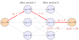
The columns are the stock levels after each period, from $x_1=0$ to $x_4=0$$0$, and the arrows join stock levels of consecutive periods; only levels 0 to 2 are drawn, and only transitions with a nonnegative order $y_i$. The highlighted route orders $2$ units in each period, and the stock goes $0\to0\to1\to0$$0$, which matches the demands $2$, $1$ and $3$. The value $f_2(1)=53$ is the cheapest cost of ending period 2 with one unit in stock; the last step adds $C_3(2)=26$ and gives $f_3(0)=79$$79$, the minimum total cost.

The upper bound $y_i\le D_i+x_{i+1}$ says exactly that the starting stock $x_i$ is not negative. The answer is $f_n(0)$ because the plan must end with $x_{n+1}=0$$0$.

This is the dynamic programming scheme with periods as stages and stock levels as states. When the cost assumptions of the zero-inventory ordering property hold, only order sizes that are sums of consecutive demands need to be tried. The highlighted route is not of this form: it carries one unit into period 3 and still orders there.

A common slip is to index $f_i$ by the starting stock $x_i$ instead of the ending stock $x_{i+1}$. The holding cost $h_ix_{i+1}$ is charged on the stock carried out of period $i$.

Key Results¶

• The bound on $y_i$ ensures nonnegative predecessor inventory.
• Reconstruct from $x_{n+1}=0$ using stored minimizers and $x_i=x_{i+1}+D_i-y_i$$y_i$.
• In the course examples, states need not exceed the remaining future demand.

Examples¶

• The three-period example gives $f_2(1)=53$ and $f_3(0)=26+53=79$$79$.
• Backward reconstruction gives $y_3=2$$2$, $x_3=1$$1$, $y_2=2$$2$, $x_2=0$$0$, $y_1=2$$2$.

Prerequisites¶

• Dynamic Programming
• Dynamic Lot-Size Model

Related Concepts¶

• Zero-Inventory Ordering Property

Sources¶

• OR Modelling · Week 6

Aliases: Dynamic lot-size recurrence, lot-size recursion Symbols: infinity

Last updated: 27 October 2026 11:52