Shadow Price in Linear Programming¶

Definition¶

The shadow price $y_i^*$ of resource $i$ is the rate of change of the optimal objective value when its right-hand side $b_i$ increases slightly. Within the applicable sensitivity range,

z^*(b_i+\Delta)=z^*(b_i)+y_i^*\Delta.

For the course's maximization LPs with $\le$ resource constraints, it equals the coefficient of slack $s_i$ in the final objective row.

Interpretation¶

A shadow price measures the marginal value of a resource: how much the optimal objective value rises per extra unit of it under the current model. Compared with the cost of acquiring the resource, buying more pays off only while the price per unit is below the shadow price.

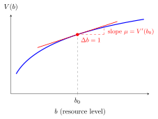
Concave value function V(b) of the resource level b, with its tangent at b0. A step of one unit in b raises the tangent by its slope, the shadow price mu.

The figure draws the optimal value $V(b)$ as a curve in the resource level $b$ . The shadow price is the slope of the line that touches the curve at the current level $b_0$ , written $\mu$ there and $y_i^*$ on this page. For an LP the curve is made of straight pieces, so within the sensitivity range the line and the curve coincide and the change $y_i^*\Delta$ in the Definition is exact rather than approximate.

The slope of $z^*(b_1)$ on the right is the shadow price $y_1^*$ . It is valid only within the range where the basis stays the same.

For maximization LPs with $\le$ resource constraints, a shadow price is never negative, since more of a resource can only enlarge the feasible region. A resource with unused slack has shadow price $0$ : extra units of something already left over cannot help. In the Giapetto model, finishing and carpentry hours both have shadow price $1$ , so one extra finishing hour raises the maximum profit from $180$ to $181$ .

A common slip is to read the shadow price as the value of the whole stock of a resource or to apply it to large changes; it is a rate, valid only over the RHS sensitivity range.

Key Results¶

The rate is valid only over its allowable right-hand-side range.
At a degenerate optimum the rates for increasing and for decreasing $b_i$ can differ, so the tableau value is then only a one-sided shadow price.
An unused resource has zero marginal value in the illustrated resource-allocation setting.
A binding constraint does not by itself guarantee a positive shadow price.
The tableau sign interpretation must be adjusted if the model or objective convention changes.

Examples¶

Malt and barley have shadow prices 1, while hops has shadow price 0 in the beer-and-ale example.
In the drinks example, an additional unit of sugar is worth 0.5 within the valid range.

Prerequisites¶

Sources¶

OR Modelling · Week 3

Aliases: dual price, dual value Keywords: shadow price Symbols: delta, mu

Last updated: 20 October 2026 03:02