Shadow Price in Constrained Optimization¶

Definition¶

In a constrained optimization problem, a shadow price is the marginal change in the optimal value when a constraint is relaxed slightly. Under the usual regularity assumptions and sign conventions, this marginal change is represented by the associated Lagrange multiplier.

For a constraint written as $g(\boldsymbol{x})=b$$b$, one commonly has

or the corresponding sign-adjusted version determined by the Lagrangian convention.

For a linear program the same quantity is the shadow price in linear programming, read off the optimal simplex tableau and valid over a right-hand-side range.

Interpretation¶

A shadow price measures how valuable a little extra room in a constraint would be at the optimum: the rate at which the optimal value changes when the right-hand side $b$ increases.

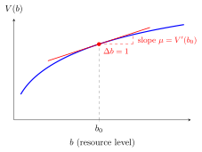
The curve is the value function $V(b)$, the optimal value for each resource level $b$, and the red line is its tangent at $b_0$. The slope of the tangent is the shadow price, written $\mu$ in the figure and $\lambda$ in the Definition. A step $\Delta b=1$ raises the tangent by $\mu$, while $V$, which bends downward here, rises a little less: the shadow price is a rate, exact only for small changes of $b$.

To see why the multiplier gives this rate, take one equality constraint $g(\boldsymbol{x})=b$ with the convention $L=f+\lambda(b-g)$$g)$, and suppose the optimizer $\boldsymbol{x}^\ast(b)$ depends differentiably on $b$. The chain rule gives $V'(b)=\boldsymbol{\nabla} f^{\top}\mathrm{d}\boldsymbol{x}^\ast/\mathrm{d}b$$\nabla f^{\top }\mathrm{d}{\mathbf{x}}^{\ast }/\mathrm{d}b$. The Lagrange condition $\boldsymbol{\nabla} f=\lambda\boldsymbol{\nabla} g$ turns this into $\lambda\,\boldsymbol{\nabla} g^{\top}\mathrm{d}\boldsymbol{x}^\ast/\mathrm{d}b$, and differentiating $g(\boldsymbol{x}^\ast(b))=b$ shows that $\boldsymbol{\nabla} g^{\top}\mathrm{d}\boldsymbol{x}^\ast/\mathrm{d}b=1$$1$. So $V'(b)=\lambda$$\lambda$, as in the envelope theorem.

The sign depends on how the constraint is written: with $L=f+\lambda(g-b)$ the same derivative is $-\lambda$. For an inequality $g(\boldsymbol{x})\le b$ in a maximization problem the multiplier is nonnegative, because extra room can never lower the maximum, and a slack constraint has shadow price $0$, as in linear programming.

A common slip is to differentiate the objective with the decision variables held fixed. For $\max xy$ subject to $x+y=b$$b$, the objective $xy$ does not even contain $b$; the shadow price $V'(b)=b/2=\lambda$$\lambda$, from $V(b)=b^2/4$ at $x=y=b/2$$b/2$, comes from reoptimizing.

Key Results¶

• A positive shadow price means relaxing the constraint raises the optimal value under the chosen convention.
• A zero shadow price often corresponds to a nonbinding inequality constraint.
• The sign depends on whether the constraint is written as a resource, residual, or equality condition.

Examples¶

• If one more unit of a resource increases maximum profit by $3$, the shadow price of that resource is $3$.
• If a budget constraint is slack, its shadow price is typically $0$ because a small increase in the budget does not improve the optimum.

Prerequisites¶

• Lagrange Multiplier
• Value Function

Related Concepts¶

• Envelope Theorem for Constrained Optimization
• Binding and Nonbinding Constraints
• Method of Lagrange for Equality Constraints

Sources¶

• Math IV: Multivariate Calculus · Week 6, Lecture 1

Keywords: shadow price, marginal value of a constraint, multiplier interpretation Symbols: delta, lambda, mu, nabla gradient

Last updated: 20 October 2026 03:02