Second-Order Sufficient Conditions for Constrained Optimization¶

Theorem¶

Let $L(\boldsymbol{x},\boldsymbol{\lambda},\boldsymbol{\mu})$ be the Lagrangian of a $C^2$ constrained problem. Consider a first-order candidate $(\boldsymbol{x}^\ast,\boldsymbol{\lambda}^\ast,\boldsymbol{\mu}^\ast)$ at which the multiplier of every binding inequality constraint is nonzero. Collect the binding inequality constraints and all equality constraints in $\boldsymbol{C}(\boldsymbol{x})$ , let $r$ be the number of active constraints (written $m$ on the bordered Hessian page, where all constraints are equalities), and assume that their gradients at $\boldsymbol{x}^\ast$ are linearly independent (nondegenerate constraint qualification, NDCQ). The relevant bordered Hessian, with $\boldsymbol{D}^2_{xx}L$ the Hessian of $L$ with respect to $\boldsymbol{x}$ , is

\boldsymbol{H}^\ast =\begin{pmatrix} \boldsymbol{0}_r & \boldsymbol{D}\boldsymbol{C}(\boldsymbol{x}^\ast)\\ \boldsymbol{D}\boldsymbol{C}(\boldsymbol{x}^\ast)^{\top} & \boldsymbol{D}^2_{xx}L(\boldsymbol{x}^\ast,\boldsymbol{\lambda}^\ast,\boldsymbol{\mu}^\ast) \end{pmatrix}.

Inspect the last $n-r$ leading principal minors after ignoring the first $2r$ leading minors. The candidate is a strict local constrained maximizer if these minors alternate in sign and the last one has sign $(-1)^n$ . It is a strict local constrained minimizer if these minors all have sign $(-1)^r$ .

Interpretation¶

The bordered Hessian checks curvature only along feasible directions. It is the constrained counterpart of using the Hessian in an unconstrained second-order test.

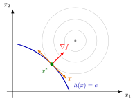
Constraint curve h(x) = c touched by a level set of f at x star, with the gradient of f perpendicular to the curve and the tangent directions T along it.

In the figure, the level set of $f$ touches the constraint curve $h(\boldsymbol{x})=c$ at the first-order candidate $\boldsymbol{x}^\ast$ , where $\boldsymbol{\nabla} f$ is parallel to $\boldsymbol{\nabla} h$ . The orange arrows mark tangent directions $T=\{\boldsymbol{v}\colon\boldsymbol{D}h(\boldsymbol{x}^\ast)\boldsymbol{v}=0\}$ $0}$ . Under the theorem's assumptions, negative curvature $\boldsymbol{v}^{\top} \boldsymbol{D}^2_{xx}L(\boldsymbol{x}^\ast,\boldsymbol{\lambda}^\ast,\boldsymbol{\mu}^\ast)\boldsymbol{v}<0$ for every nonzero feasible tangent direction gives a strict local constrained maximum; positive curvature gives a strict local constrained minimum. For multiple active constraints, use $T=\ker \boldsymbol{D}\boldsymbol{C}(\boldsymbol{x}^\ast)$ and the bordered-Hessian sign test above.

The mixed-constraint Lagrange method supplies the first-order candidate and its multipliers. The second-order test then examines the Lagrangian curvature on the feasible tangent directions, under the strict active-multiplier and regularity hypotheses stated above.

Key Results¶

Only binding inequality constraints and equality constraints enter the relevant bordered Hessian.
The nonzero multipliers on binding inequality constraints are part of the theorem, so check them before applying the test. If a binding inequality has a zero multiplier, the test does not apply.
The theorem gives sufficient conditions for strict local constrained optima.
Zero or semidefinite cases can be inconclusive.

Examples¶

With one equality constraint in two variables, the relevant bordered Hessian is a three-by-three matrix.
For a maximization problem with three variables and one active constraint, the final relevant determinant must have sign $(-1)^3$ .

Prerequisites¶

Sources¶

Math IV: Multivariate Calculus · Week 6, Lecture 2

Keywords: constrained SOSC, bordered Hessian sufficient conditions Symbols: lambda, mu, nabla gradient

Last updated: 22 October 2026 19:04