Hessian Matrix¶

Definition¶

Let $f\colon E\subseteq\mathbb{R}^n\to\mathbb{R}$ be a scalar-valued function whose second-order partial derivatives exist at $\boldsymbol{x}_0\in E$ $E$ . The Hessian matrix of $f$ at $\boldsymbol{x}_0$ is

\boldsymbol{H}_f(\boldsymbol{x}_0) =\begin{pmatrix} \frac{\partial^2 f}{\partial x_1^2}(\boldsymbol{x}_0) & \cdots & \frac{\partial^2 f}{\partial x_1\partial x_n}(\boldsymbol{x}_0)\\ \vdots & \ddots & \vdots\\ \frac{\partial^2 f}{\partial x_n\partial x_1}(\boldsymbol{x}_0) & \cdots & \frac{\partial^2 f}{\partial x_n^2}(\boldsymbol{x}_0) \end{pmatrix}.

The entry in row $i$ and column $j$ is the second partial derivative with respect to $x_i$ and $x_j$ .

Interpretation¶

The Hessian collects all second-order bending information of a scalar function at one point. It is the multivariable analogue of the second derivative in one-variable calculus.

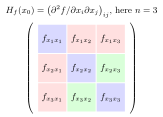
The 3 by 3 Hessian matrix of second partial derivatives, with pure second partials on the diagonal and mixed partials, equal in symmetric pairs, off the diagonal.

The blue diagonal entries are the pure second partials, measuring curvature along the coordinate axes. The mixed partials appear in symmetric pairs when $f$ is $C^2$ . When $f$ is $C^2$ on an open neighbourhood of $\boldsymbol{x}_0$ , the second-order approximation is $f(\boldsymbol{x}_0+\boldsymbol{h})=f(\boldsymbol{x}_0)+\boldsymbol{\nabla} f(\boldsymbol{x}_0)\cdot \boldsymbol{h}+\frac{1}{2}\boldsymbol{h}^{\top} \boldsymbol{H}_f(\boldsymbol{x}_0)\boldsymbol{h}+o(\|\boldsymbol{h}\|^2)$ $o (∥ h ∥^{2})$ . At a stationary point, positive or negative definiteness gives a strict local minimum or maximum, and an indefinite Hessian gives a saddle; semidefinite cases can be inconclusive.

Drag $\boldsymbol{x}_0$ : the Hessian collects the second-order partial derivatives there, and its eigenvalues describe how the level curves bend.

Move $\boldsymbol{x}_0$ and read $\boldsymbol{H}_f(\boldsymbol{x}_0)$ : at the marked critical points its definiteness matches the shape of the surface.

Arranging the second derivatives in a matrix makes curvature along a displacement accessible through the quadratic form $\boldsymbol{h}^{\top}\boldsymbol{H}_f\boldsymbol{h}$ . For a $C^2$ function, this is the second-order term in the local Taylor approximation, up to its factor $1/2$ .

Key Results¶

For the second-order tests below, assume $f$ is $C^2$ on an open neighbourhood of $\boldsymbol{x}_0$ and $\boldsymbol{\nabla}f(\boldsymbol{x}_0)=\boldsymbol{0}$ $0$ . Mere existence of the Hessian at one point is insufficient.

If $f$ is $C^2$ near $\boldsymbol{x}_0$ , then the Hessian is symmetric.
At a critical point (for differentiable $f$ the same as a stationary point, $\boldsymbol{\nabla}f(\boldsymbol{x}_0)=\boldsymbol{0}$ $0$ ), a positive definite Hessian gives a strict local minimum.
At a critical point, a negative definite Hessian gives a strict local maximum.
At a critical point, an indefinite Hessian gives a saddle point.

Examples¶

For $f(x,y)=x^2+2xy+3y^2$ $3 y^{2}$ , the Hessian is $\begin{pmatrix}2&2\\2&6\end{pmatrix}$ at every point.
For $f(x,y)=x^3+2xy^2-y^3$ $y^{3}$ , the Hessian at $(1,1)$ is $\begin{pmatrix}6&4\\4&-2\end{pmatrix}$ .

Prerequisites¶

Sources¶

Math IV: Multivariate Calculus · Week 1, Lecture 1

Aliases: Hessian, second derivative matrix, Hessian matrix of a function, Hesse matrix Keywords: matrix of second partial derivatives Symbols: element of, nabla gradient, partial, real numbers, subset

Last updated: 22 October 2026 19:04