Lagrange Multiplier¶

Definition¶

A Lagrange multiplier is an auxiliary variable attached to a constraint in a Lagrangian. For equality constraints $h_j(\boldsymbol{x})=c_j$ $c_{j}$ , a typical course convention writes

L(\boldsymbol{x},\boldsymbol{\mu})=f(\boldsymbol{x})+\sum_{j=1}^m\mu_j(c_j-h_j(\boldsymbol{x})).

At a regular constrained optimum, the multipliers make the gradient of the objective a linear combination of the gradients of the active constraints.

Interpretation¶

A multiplier records how a constraint enters the first-order trade-off at a candidate optimum. In parameterized problems, it can also measure the marginal value of relaxing a constraint.

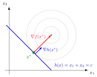
Circular level sets of f and the constraint line x1 + x2 = c. At the optimum x star the level set touches the line, and the gradient of f is a multiple of the gradient of the constraint.

At the illustrated optimum, $\boldsymbol{\nabla} f(\boldsymbol{x}^\ast)=\mu\boldsymbol{\nabla} h(\boldsymbol{x}^\ast)$ $μ \nabla h (x^{*})$ , so the level set of $f$ is tangent to the constraint curve. The figure maximizes $f(\boldsymbol{x})=-(x_1-3)^2-(x_2-2.5)^2$ $2.5)^{2}$ , whose level sets are circles about $(3,2.5)$ , subject to $x_1+x_2=3$ $3$ . The optimum is $\boldsymbol{x}^\ast=(1.75,1.25)$ $(1.75, 1.25)$ , where $\boldsymbol{\nabla} f(\boldsymbol{x}^\ast)=(2.5,2.5)=2.5\,\boldsymbol{\nabla} h(\boldsymbol{x}^\ast)$ $2.5 \nabla h (x^{*})$ , so $\mu=2.5$ $2.5$ . Under the sensitivity assumptions stated for the envelope theorem, $\mu=\mathrm{d}V/\mathrm{d}c$ measures the marginal value of changing the constraint level. In the figure, the optimal value for level $c$ is $V(c)=-\tfrac{1}{2}(5.5-c)^2$ $c)^{2}$ , and $V'(3)=2.5=\mu$ $μ$ .

Move the point until the arrows $\boldsymbol{\nabla} f$ and $\boldsymbol{\nabla} h$ line up (both are drawn to the same scale). The factor between them is the multiplier $\mu$ .

Key Results¶

Equality multipliers may be positive, negative, or zero.
Inequality multipliers have sign restrictions under the course convention.
In the envelope theorem, some multipliers can be interpreted as shadow prices.

Examples¶

Maximize $xy$ subject to $x+y=10$ $10$ . With $L(x,y,\mu)=xy+\mu(10-x-y)$ $y)$ , stationarity gives $y-\mu=0$ and $x-\mu=0$ $0$ , so $x=y=\mu$ $μ$ ; the constraint then gives $x=y=5$ and $\mu=5$ $5$ , with maximum $25$ . Raising the budget from $10$ to $11$ raises the maximum to $5.5^2=30.25$ $30.25$ , an increase of $5.25\approx\mu$ $μ$ : the multiplier is the marginal value of the budget.
Minimize $x^2+y^2$ subject to $x+y=1$ $1$ . For $L(x,y,\mu)=x^2+y^2+\mu(1-x-y)$ $y)$ , stationarity gives $2x-\mu=0$ and $2y-\mu=0$ $0$ , so $x=y=\mu/2$ $μ /2$ . The constraint gives $\mu=1$ and $x=y=\tfrac{1}{2}$ $\frac{1}{2}$ , with minimum value $\tfrac{1}{2}$ . For level $c$ the minimum is $c^2/2$ , whose derivative at $c=1$ is $1=\mu$ $μ$ .

Prerequisites¶

Sources¶

Math IV: Multivariate Calculus · Week 4, Lecture 2
Math IV: Multivariate Calculus · Week 6, Lecture 1

Aliases: Kuhn-Tucker multiplier, KKT multiplier Keywords: multiplier, constraint multiplier, lambda multiplier, mu multiplier Symbols: mu, nabla gradient, sum

Last updated: 17 October 2026 21:53