Implicit Function Theorem¶

Theorem¶

In a system $\boldsymbol{G}(\boldsymbol{x},\boldsymbol{y})=0$ $0$ , the variables $\boldsymbol{x}\in\mathbb{R}^n$ are treated as exogenous and $\boldsymbol{y}\in\mathbb{R}^m$ as endogenous. For $\boldsymbol{G}\colon A\to\mathbb{R}^m$ $R^{m}$ , define the partial Jacobians $\boldsymbol{D}_x\boldsymbol{G}$ and $\boldsymbol{D}_y\boldsymbol{G}$ by differentiating with respect to the $\boldsymbol{x}$ -block and $\boldsymbol{y}$ -block.

Let $A\subseteq\mathbb{R}^{n+m}$ be open and let $\boldsymbol{G}\colon A\to\mathbb{R}^m$ be $C^1$ . Suppose $(\boldsymbol{x}_0,\boldsymbol{y}_0)\in A$ $A$ , $\boldsymbol{G}(\boldsymbol{x}_0,\boldsymbol{y}_0)=0$ $0$ , and

\det(\boldsymbol{D}_y\boldsymbol{G}(\boldsymbol{x}_0,\boldsymbol{y}_0))\neq 0.

Then there is a neighbourhood $B$ of $\boldsymbol{x}_0$ and a $C^1$ function $\boldsymbol{\varphi}\colon B\to\mathbb{R}^m$ such that $\boldsymbol{\varphi}(\boldsymbol{x}_0)=\boldsymbol{y}_0$ and $\boldsymbol{G}(\boldsymbol{x},\boldsymbol{\varphi}(\boldsymbol{x}))=0$ for all $\boldsymbol{x}\in B$ $B$ . After shrinking $B$ if necessary, there is a neighbourhood $W$ of $\boldsymbol{y}_0$ such that, for each $\boldsymbol{x}\in B$ $B$ , $\boldsymbol{y}=\boldsymbol{\varphi}(\boldsymbol{x})$ is the only solution of $\boldsymbol{G}(\boldsymbol{x},\boldsymbol{y})=0$ in $W$ . Moreover,

\boldsymbol{D}\boldsymbol{\varphi}(\boldsymbol{x}_0) =-(\boldsymbol{D}_y\boldsymbol{G}(\boldsymbol{x}_0,\boldsymbol{y}_0))^{-1}\boldsymbol{D}_x\boldsymbol{G}(\boldsymbol{x}_0,\boldsymbol{y}_0).

For one equation in two variables, this reduces to $\varphi'(x_0)=-G_x(x_0,y_0)/G_y(x_0,y_0)$ $- G_{x} (x_{0}, y_{0}) / G_{y} (x_{0}, y_{0})$ .

Interpretation¶

The theorem says that a regular system of equations can locally be solved for the variables that must adjust. It also gives the local response of those adjusting variables when the chosen variables change.

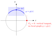
Unit circle x^2 + y^2 = 1 with a window around (0, 1) in which the circle is the graph of y = g(x). At (1, 0) the tangent is vertical and no such local graph exists.

For the circle $G(x,y)=x^2+y^2-1=0$ $0$ , the point $(x_0,y_0)=(0,1)$ has $G_y(x_0,y_0)=2\ne0$ $0$ . In a neighbourhood of that point, the circle is the graph $y=g(x)=\sqrt{1-x^2}$ $1 - x^{2}$ , and $g'(x)=-x/y$ $- x / y$ . The theorem above gives the corresponding derivative formula for systems of equations.

Move along $x^2+y^2=1$ $1$ : wherever $D_yG\ne0$ the curve is locally a graph $y=\varphi(x)$ with slope $-D_xG/D_yG$ . At $y=0$ this fails.

The Jacobian contains the first-order effects of the equation variables. Its endogenous block must be invertible to solve locally for changes in the endogenous variables; a singular block does not meet the theorem's hypothesis.

Key Results¶

The determinant condition says the endogenous block is locally pinned down by the equations.
The theorem gives local existence, differentiability, and a derivative formula.
The one-equation case is the familiar slope formula for an implicit curve.

Examples¶

For $G(x,y)=y-x^2$ $x^{2}$ , the theorem gives $y=\varphi(x)=x^2$ because $D_yG=1$ $1$ .
For $G(x,y)=x^2+y^2-1$ near $(0,1)$ , the theorem gives the upper circle locally as a function of $x$ .

Prerequisites¶

Sources¶

Math IV: Multivariate Calculus · Week 2, Lecture 2

Keywords: multivariable implicit function theorem, implicit derivative formula, IFT, partial Jacobians Symbols: element of, phi, real numbers, square root, subset

Last updated: 22 October 2026 19:04