Multivariate Taylor Approximations¶

Definition¶

Let $f\colon\mathbb{R}^n\to\mathbb{R}$ be sufficiently smooth near $\boldsymbol{x}_0$ and let $\boldsymbol{h}$ be a small displacement. The first-order Taylor approximation is

f(\boldsymbol{x}_0+\boldsymbol{h})\approx f(\boldsymbol{x}_0)+\boldsymbol{D}f(\boldsymbol{x}_0)\boldsymbol{h}.

If $f$ is $C^2$ near $\boldsymbol{x}_0$ , the second-order approximation is

f(\boldsymbol{x}_0+\boldsymbol{h})\approx f(\boldsymbol{x}_0)+\boldsymbol{D}f(\boldsymbol{x}_0)\boldsymbol{h} +\frac{1}{2} \boldsymbol{h}^{\top} \boldsymbol{H}_f(\boldsymbol{x}_0)\boldsymbol{h}.

The first correction uses local slope, and the second correction uses local curvature.

Interpretation¶

Taylor approximations replace a complicated function near a point by simpler local information. The linear term estimates the immediate change, and the quadratic term corrects for bending.

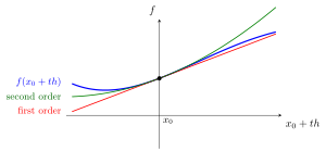
A function along a line through x0 together with its first-order (straight-line) approximation and its second-order (parabolic) approximation, all touching at x0.

The figure follows the line $\boldsymbol{x}_0+t\boldsymbol{h}$ for a fixed direction $\boldsymbol{h}$ . Its first-order approximation is $f(\boldsymbol{x}_0)+t\boldsymbol{D}f(\boldsymbol{x}_0)\boldsymbol{h}$ $t D f (x_{0}) h$ ; the second-order approximation adds $\frac{1}{2}t^2\boldsymbol{h}^{\top}\boldsymbol{H}_f(\boldsymbol{x}_0)\boldsymbol{h}$ . As $t\to0$ $0$ , the errors are $o(|t|)$ under differentiability and $o(t^2)$ under the $C^2$ hypothesis.

Compare both approximations along a line through $\boldsymbol{x}_0$ (right). Under the smoothness assumptions, the Hessian term improves the order of the local error as the displacement tends to zero.

Compare the first-order approximation (the tangent plane) with the second-order one, $f(\boldsymbol{x}_0)+\boldsymbol{D}f(\boldsymbol{x}_0)\boldsymbol{h}+\tfrac{1}{2}\boldsymbol{h}^{\top}\boldsymbol{H}_f(\boldsymbol{x}_0)\boldsymbol{h}$ $\frac{1}{2} h^{⊤} H_{f} (x_{0}) h$ , near $\boldsymbol{x}_0$ .

The Jacobian of a scalar-valued function is a row matrix, so multiplying it by the displacement gives the first-order scalar change. The Hessian contributes the quadratic correction when the $C^2$ hypothesis holds.

Key Results¶

For a real-valued function, $\boldsymbol{D}f(\boldsymbol{x}_0)\boldsymbol{h}=\boldsymbol{\nabla} f(\boldsymbol{x}_0)^{\top} \boldsymbol{h}$ $\nabla f (x_{0})^{⊤} h$ .
If $f$ is $C^2$ , then the Hessian is symmetric and the second-order term is a quadratic form.
At a critical point, the quadratic term is the first potentially nonzero correction. It may also vanish, in which case higher-order information is needed.

Examples¶

For $f(x,y)=x^2+xy+y^2$ at $(0,0)$ , the second-order approximation is exact.
For $f(x,y)=\mathrm{e}^{x+y}$ at $(0,0)$ , the second-order approximation is $1+x+y+\frac{1}{2}(x+y)^2$ $y)^{2}$ .

Prerequisites¶

Sources¶

Math IV: Multivariate Calculus · Week 2, Lecture 1

Aliases: multivariate Taylor expansion Keywords: linear approximation in Rn, second-order approximation, quadratic approximation, Taylor approximation with Hessian Symbols: nabla gradient, real numbers

Last updated: 22 October 2026 19:04