Envelope Theorem for Constrained Optimization¶

Theorem¶

In a parametric problem, the value function is the optimized objective value

F(\boldsymbol{\alpha})=f(\boldsymbol{\gamma}(\boldsymbol{\alpha});\boldsymbol{\alpha}),

where $\boldsymbol{\gamma}(\boldsymbol{\alpha})$ is an optimizer. For equality constraints, define

L(\boldsymbol{x},\boldsymbol{\mu};\boldsymbol{\alpha})=f(\boldsymbol{x};\boldsymbol{\alpha})+\sum_j\mu_jh_j(\boldsymbol{x};\boldsymbol{\alpha}).

If smooth optimizer and multiplier functions satisfy the first-order conditions, then

\frac{\partial F}{\partial\alpha_\ell}(\boldsymbol{\alpha})=\frac{\partial L}{\partial\alpha_\ell}\big(\boldsymbol{\gamma}(\boldsymbol{\alpha}),\widetilde{\boldsymbol{\mu}}(\boldsymbol{\alpha});\boldsymbol{\alpha}\big).

For mixed constraints, the same formula holds with the Lagrangian including the binding inequalities and equality constraints, provided the relevant bordered Hessian is nonsingular and the active set is smooth. In the special equality case $h_j(\boldsymbol{x};\boldsymbol{\alpha})=\alpha_j-\widetilde h_j(\boldsymbol{x})$ with $f$ independent of $\boldsymbol{\alpha}$ , the multiplier is the shadow price:

\frac{\partial F}{\partial\alpha_j}(\boldsymbol{\alpha})=\widetilde\mu_j(\boldsymbol{\alpha}).

Interpretation¶

The envelope theorem computes how the best attainable value changes when a parameter changes. It avoids separately differentiating every movement of the optimizer.

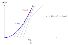
The value function V(alpha) drawn as the upper envelope of grey curves alpha to f(x; alpha), one for each fixed x. At alpha0 the envelope touches one curve and has the same slope.

In the illustrated example, the feasible choices do not depend on $\alpha$ , and the value function $V(\alpha)=\max_x f(x;\alpha)$ (written $F$ in the theorem above) is the upper envelope of the grey curves obtained by fixing $x$ . At $\alpha_0$ , it touches the curve for $x^\ast(\alpha_0)$ and shares its slope: $V'(\alpha_0)=\frac{\partial f}{\partial\alpha}(x^\ast(\alpha_0);\alpha_0)$ $\frac{\partial f}{\partial α} (x^{*} (α_{0}); α_{0})$ . The theorem above gives the corresponding formula when the constraints depend on the parameter.

The derivative of the optimal value $F(\alpha)$ equals the partial derivative of the Lagrangian with respect to $\alpha$ at the optimum, here the multiplier $\mu$ .

The equality-constraint Lagrange method supplies the stationarity equations. Applying the implicit function theorem to those equations and the constraints can give locally smooth optimizer and multiplier functions when the relevant bordered Hessian is nonsingular. The chain-rule terms involving optimizer movements then cancel by stationarity and differentiated feasibility.

Key Results¶

The value function records the optimum as a function of parameters.
The envelope derivative is the direct parameter derivative of the Lagrangian at the optimal solution.
A shadow price is the marginal value of relaxing a constraint in the stated equality-constraint setup.

Examples¶

For $f(x;\alpha)=\alpha x-x^2$ $x^{2}$ , the envelope derivative is $x^\ast(\alpha)$ .
In utility maximization with income as a parameter, the multiplier on the budget equation measures marginal utility of income.

Prerequisites¶

Sources¶

Math IV: Multivariate Calculus · Week 6, Lecture 1
Math IV: Multivariate Calculus · Week 7, Lecture 1

Keywords: envelope theorem, equality envelope theorem, mixed-constraint envelope theorem, value function, shadow price Symbols: alpha, gamma, mu, partial, sum

Last updated: 26 October 2026 00:09