Objective Coefficient Range¶

Definition¶

An objective coefficient range is an interval of values for one objective coefficient over which the current optimal basis remains optimal while all other data stay fixed. A report with coefficient $c_j$, allowable decrease $d_j$, and allowable increase $u_j$ gives

Interpretation¶

The objective coefficient range answers how far one profit or cost coefficient may move before a different decision becomes optimal. Within this interval the reported decision stays an optimum; only its objective value changes, because the same quantities now earn a different return per unit.

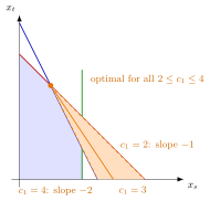
With objective $c_1x_s+2x_t$$2x_t$, every objective line has slope $-c_1/2$. The corner $(20,60)$ stays optimal as long as this slope lies between the slopes of the two constraint lines through it: $-1$ for carpentry, $x_s+x_t\le80$$80$, and $-2$ for finishing, $2x_s+x_t\le100$$100$. That gives $1\le c_1/2\le2$$2$, the range $2\le c_1\le4$ shaded as a fan. At $c_1=2$ or $c_1=4$ the objective line lies along an edge of the region, and the whole edge is optimal.

The range is a one-at-a-time question of sensitivity analysis, stated in the Excel sensitivity report as an allowable decrease and increase. For a variable that is $0$ at the optimum, lowering its coefficient never makes it attractive, so the decrease is unlimited; for a nonbasic variable the allowable increase equals the size of its reduced cost.

Separate ranges do not combine. Raising $c_1$ to $4$ and lowering the train coefficient from $2$ to $1.6$ stays within each range on its own, but together the slope is $-2.5$, steeper than the finishing line, and the optimum moves to $(40,20)$.

Key Results¶

• For a change $\Delta c_j$ within the range, the value changes by $x_j^*\Delta c_j$.
• At a range endpoint, additional optimal solutions may become available.
• Separate reported ranges do not justify simultaneous changes automatically.

Examples¶

For the illustrated objective $c_1x_s+2x_t$$2x_t$, the coefficient $c_1=3$ may decrease or increase by 1, giving $[2,4]$. The corner $(20,60)$ remains optimal, while its value becomes $20c_1+120$$120$; endpoint values may admit other optima.

• The small-pipe profit coefficient 5 has allowable decrease 1 and increase 3, giving $[4,8]$.
• Changing banana profit by $-0.03$ with quantity 75 changes total profit by $-2.25$.

Prerequisites¶

• Sensitivity Analysis
• Objective Function

Related Concepts¶

• Reduced Cost
• RHS Sensitivity Range

Sources¶

• OR Modelling · Week 3

Aliases: range of optimality, optimality range, cost coefficient range Symbols: delta

Last updated: 20 October 2026 03:02