Poisson Distribution¶

Definition¶

Let $\lambda>0$ $0$ . A discrete random variable $X$ has a Poisson distribution with parameter $\lambda$ , written $X\sim\operatorname{Pois}(\lambda)$ $Pois (λ)$ , if, for $k=0,1,2,\ldots$ $0, 1, 2, \dots$ ,

\mathbb{P}(X=k)=\mathrm{e}^{-\lambda}\frac{\lambda^k}{k!},

and the PMF is zero elsewhere. The extension $\lambda=0$ gives the constant-zero distribution.

Interpretation¶

A Poisson variable models a count of events in a fixed period, such as arrivals or claims, when there is no fixed upper limit on the count. Its single parameter $\lambda$ is the mean count.

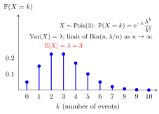
Probability bars of the Poisson(3) distribution for 0 to 10 events, with the highest bars at 2 and 3 and the mean 3 marked.

The figure shows $\operatorname{Pois}(3)$ . The bars at $2$ and $3$ are equally high, $\tfrac{9}{2}\mathrm{e}^{-3}\approx0.224$ $0.224$ , and the bars fall off quickly on both sides: the values above $10$ have total probability below $0.001$ . The mean $\lambda=3$ is marked.

Change $\lambda$ : it is both the mean and the variance. Small $\lambda$ piles the mass near $0$ ; large $\lambda$ gives a wider, more symmetric hump.

The ratio of neighbouring masses explains the shape: $\mathbb{P}(X=k)/\mathbb{P}(X=k-1)=\lambda/k$ $λ / k$ , so the bars increase while $k<\lambda$ and decrease once $k>\lambda$ $λ$ . When $\lambda$ is an integer, as here, the two bars at $\lambda-1$ and $\lambda$ are equal. The factorial makes the masses eventually shrink faster than any geometric sequence, and they add up to $1$ because $\displaystyle \sum_{k\ge0}\lambda^k/k!=\mathrm{e}^{\lambda}$ $e^{λ}$ , the series of the exponential function.

The Poisson distribution approximates the binomial distribution with many trials and a small success probability: for large $n$ , $\operatorname{Bin}(n,\lambda/n)$ is close to $\operatorname{Pois}(\lambda)$ , as the Further Properties state. This is why it fits counts of rare events among many independent opportunities. The same distribution describes the number of arrivals in an interval of a Poisson process.

The parameter is also the variance, so a Poisson model fixes the spread once the mean is known. Count data whose variance is clearly larger than the mean are therefore not well described by a single Poisson distribution.

Key Results¶

$\mathbb{E}X=\operatorname{Var}(X)=\lambda$ $λ$ .
MGF $M_X(t)=\exp(\lambda(\mathrm{e}^t-1))$ for every real $t$ .

Examples¶

For $\lambda=2$ $2$ , $\mathbb{P}(X=0)=\mathrm{e}^{-2}$ and $\mathbb{P}(X=1)=2\mathrm{e}^{-2}$ $2 e^{- 2}$ .
A Poisson count with mean $5$ has variance $5$ and standard deviation $\sqrt{5}$ .

Further Properties¶

Independent Poisson counts add to a Poisson count with the sum of their parameters. A binomial model converges to this law when the number of trials tends to infinity and the success probabilities shrink so that their product tends to a fixed parameter.

Prerequisites¶

Sources¶

Probability Theory for EOR · Week 4
Nicky van Foreest · Probability Distributions · Refresher

Aliases: Pois(lambda), Poisson random variable, Poisson r.v., Poisson variable Symbols: lambda, square root, sum

Last updated: 20 October 2026 03:02