Standard Normal Distribution¶

Definition¶

A random variable $Z$ has the standard normal distribution, written $Z\sim\mathcal{N}(0,1)$ $N (0, 1)$ , if its density is $\phi$ ; its CDF is $\Phi$ :

\phi(z)=\frac{1}{\sqrt{2\pi}}\mathrm{e}^{-z^2/2},\qquad \Phi(z)=\int_{-\infty}^z\phi(t)\,\mathrm{d}t.

In $\mathcal{N}(\mu,\sigma^2)$ the second parameter is the variance.

Interpretation¶

The standard normal distribution is the single reference bell curve, centred at $0$ with variance $1$ . Every normal probability can be read from its CDF $\Phi$ , because any normal variable becomes standard normal after standardization: a value is then measured in standard deviations from the mean.

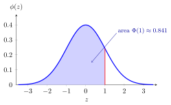
The standard normal density with the area to the left of z = 1 shaded, equal to about 0.841.

The shaded area is everything to the left of $z=1$ $1$ , that is $\Phi(1)=\mathbb{P}(Z\le1)\approx0.841$ $0.841$ , the first Example. The unshaded right tail has area $1-\Phi(1)\approx0.159$ $0.159$ . Since $\phi$ is symmetric about $0$ , the left tail below $-1$ has the same area, so $\Phi(-1)=1-\Phi(1)$ and $\mathbb{P}(-1\le Z\le1)=2\Phi(1)-1\approx0.683$ $0.683$ .

Move $c$ and $d$ and read probabilities as differences $\Phi(d)-\Phi(c)$ $Φ (c)$ ; try $c=-1.96$ $- 1.96$ , $d=1.96$ $1.96$ .

The density $\phi$ has no antiderivative in terms of elementary functions, so $\Phi$ is evaluated numerically, by a table or software. A table for $z\ge0$ suffices: symmetry gives $\Phi(-z)=1-\Phi(z)$ $Φ (z)$ , and interval probabilities are differences $\Phi(d)-\Phi(c)$ $Φ (c)$ . The value $1.96$ suggested in the manipulate prompt satisfies $\Phi(1.96)\approx0.975$ $0.975$ , so $\mathbb{P}(-1.96\le Z\le1.96)\approx0.95$ $0.95$ .

For $Y\sim\mathcal{N}(\mu,\sigma^2)$ $N (μ, σ^{2})$ , the variable $(Y-\mu)/\sigma$ is standard normal, so $\mathbb{P}(Y\le y)=\Phi\big((y-\mu)/\sigma\big)$ $μ) / σ)$ ; the second Example uses this with $\mu=10$ and $\sigma=2$ $2$ . A common slip is to divide by the variance: in $\mathcal{N}(10,4)$ the second parameter is $\sigma^2=4$ $4$ , so the divisor is $\sigma=2$ $2$ . Later, sums of many independent variables are approximated by this distribution after standardization, in the central limit theorem.

Key Results¶

$\mathbb{E}Z=0$ $0$ , $\operatorname{Var}(Z)=1$ $1$ , and $\Phi(-z)=1-\Phi(z)$ $Φ (z)$ .
If $Y\sim\mathcal{N}(\mu,\sigma^2)$ with $\sigma>0$ $0$ , then $(Y-\mu)/\sigma\sim\mathcal{N}(0,1)$ $N (0, 1)$ .
Quantiles transform the same way: the $p$ -quantile of $Y$ is $\mu+\sigma\Phi^{-1}(p)$ $σ Φ^{- 1} (p)$ . Printed normal tables list the left-tail probabilities $\Phi(z)$ , so a quantile is read off the table in reverse and then transformed back.

Examples¶

$\mathbb{P}(Z\le1)=\Phi(1)\approx0.8413$ $0.8413$ .
For $Y\sim\mathcal{N}(10,4)$ $N (10, 4)$ , $\mathbb{P}(Y\le12)=\Phi((12-10)/2)=\Phi(1)\approx0.8413$ $0.8413$ .

Prerequisites¶

Normal Distribution

Sources¶

Probability Theory for EOR · Week 5
Probability Distributions · supporting concept
OR Modelling · Week 6

Aliases: N(0,1), standard Gaussian, standard normal, unit normal distribution, standard normal random variable, standard Gaussian distribution Symbols: infinity, integral, mu, phi, pi, sigma, square root

Last updated: 22 October 2026 19:04