Rayleigh Distribution¶

Definition¶

Let $\sigma>0$ $0$ . A continuous random variable $X$ has a Rayleigh distribution with parameter $\sigma$ if its density is

f_X(x)=\frac{x}{\sigma^2}\exp\left(-\frac{x^2}{2\sigma^2}\right),

for $x\ge 0$ $0$ , and $f_X(x)=0$ for $x<0$ $0$ .

Interpretation¶

The Rayleigh distribution describes a nonnegative distance: typically the distance from the origin of a random point $(Y_1,Y_2)$ in the plane whose two coordinates are independent and normal with mean $0$ and the same variance $\sigma^2$ . The Euclidean distance $X=\sqrt{Y_1^2+Y_2^2}$ then has the density of the Definition.

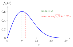
A Rayleigh density rising from 0 to a peak at sigma and then decaying, with dashed lines at the mode sigma and the mean, about 1.25 sigma.

The figure shows the density for $\sigma=1$ $1$ , with the horizontal axis in multiples of $\sigma$ . It starts at $0$ , because a distance near $0$ requires both coordinates to be near $0$ . It rises to its peak at $x=\sigma$ (the green line, labelled mode) and then falls quickly, because of the factor $\exp(-x^2/(2\sigma^2))$ . The red line marks the mean $\sigma\sqrt{\pi/2}\approx1.25\sigma$ $1.25 σ$ , to the right of the peak, since the right side of the curve is longer than the left side.

Change $\sigma$ : the density peaks at $x=\sigma$ and the mean sits a little further out, at $\sigma\sqrt{\pi/2}$ .

Unlike the normal density, this density can be integrated by hand: $x/\sigma^2$ is, up to sign, the derivative of the exponent, so substitution gives, for $x\ge0$ $0$ ,

F_X(x)=1-\exp\left(-\frac{x^2}{2\sigma^2}\right).

So $\mathbb{P}(X>x)=\exp(-x^2/(2\sigma^2))$ $exp (- x^{2} / (2 σ^{2}))$ , and probabilities are density integrals over nonnegative intervals, as for any continuous random variable. The parameter $\sigma$ only sets the scale: $X/\sigma$ has the Rayleigh distribution with parameter $1$ . Note that $\sigma$ is the standard deviation of each coordinate $Y_i$ , not of $X$ itself.

In one dimension the corresponding distance $|Y_1|$ from the origin has a folded normal distribution.

Key Results¶

The Rayleigh distribution is supported on nonnegative values.
It arises as the magnitude of a two-dimensional random vector with independent, centred normal components of equal variance.
Its density starts at zero, rises to a peak, and then decays.

Examples¶

Wind speed magnitude can sometimes be modelled with a Rayleigh distribution.
The distance error from two independent normal coordinate errors can be Rayleigh.
Signal envelope amplitudes in some noise models follow a Rayleigh distribution.

Prerequisites¶

Continuous Random Variable

Sources¶

Probability Theory for EOR · Week 5

Aliases: Rayleigh law, Rayleigh random variable Symbols: pi, sigma, square root

Last updated: 20 October 2026 03:02