Binomial Distribution¶

Definition¶

Let $n$ be a nonnegative integer, $0\le p\le1$ and $q=1-p$ $p$ . A discrete random variable $X$ has a binomial distribution with parameters $n$ and $p$ , written $X\sim\operatorname{Bin}(n,p)$ $Bin (n, p)$ , if

\begin{gathered} \mathbb{P}(X=k)=\binom{n}{k}p^kq^{n-k},\\ k=0,1,\ldots,n, \end{gathered}

and the PMF is zero elsewhere. Equivalently, $X$ is the sum of $n$ i.i.d. Bernoulli variables with success probability $p$ .

Interpretation¶

A binomial variable counts the successes in a fixed number $n$ of independent trials that each succeed with the same probability $p$ .

Probability bars of the Binomial(10, 0.3) distribution for 0 to 10 successes, peaking at 3, which is also the mean.

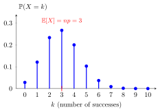
The figure shows $X\sim\operatorname{Bin}(10,0.3)$ $Bin (10, 0.3)$ , the number of successes in ten trials with success probability $0.3$ . The bars give $\mathbb{P}(X=k)=\binom{10}{k}0.3^k0.7^{10-k}$ for $k=0,\ldots,10$ $0, \dots, 10$ . The tallest bar is at $k=3$ $3$ , with probability about $0.27$ , and the bars for $k\ge8$ are nearly invisible: together they have probability about $0.0016$ . The marked value $np=3$ is the mean of the distribution: in ten trials with success probability $0.3$ , about three successes are typical.

Change $n$ and $p$ : the bars sit around $\mathbb{E}X=np$ with spread $\sqrt{npq}$ . Use $c$ and $d$ to add up $\mathbb{P}(c\le X\le d)$ $d)$ , and hover over a bar for its formula.

The PMF has two factors. Each trial is a Bernoulli trial, and by independence any one fixed sequence with $k$ successes and $n-k$ failures, such as $k$ successes followed by $n-k$ failures, has probability $p^kq^{n-k}$ . The binomial coefficient $\binom nk$ counts how many such sequences there are, one for each choice of the $k$ positions of the successes. Forgetting it is a common slip: for three fair tosses, $\mathbb{P}(X=2)=\binom32\cdot\tfrac{1}{8}=\tfrac{3}{8}$ $\frac{3}{8}$ , not $\tfrac{1}{8}$ .

All three conditions matter. When the draws are made without replacement from a small population, the trials are not independent and the count is hypergeometric instead. When the number of trials is not fixed but one waits for the first success, the first success distribution applies.

Key Results¶

$\mathbb{E}X=np$ and $\operatorname{Var}(X)=np(1-p)$ $p)$ .
MGF $M_X(t)=(1-p+p\mathrm{e}^t)^n$ $p e^{t})^{n}$ .

Examples¶

For three fair tosses, $\mathbb{P}(X=2)=\binom32(1/2)^3=3/8$ $3/8$ .
For $n=10$ $10$ , $p=0.2$ $0.2$ , the count has mean $2$ , variance $1.6$ , and no-success probability $0.8^{10}$ .

Further Properties¶

The binomial count is a sum of independent Bernoulli trials. In the rare-event limit $n\to\infty$ $\infty$ , $p_n\to0$ $0$ , and $np_n\to\lambda$ $λ$ , its distribution converges to $\operatorname{Pois}(\lambda)$ .

Prerequisites¶

Sources¶

Probability Theory for EOR · Week 3
Nicky van Foreest · Probability Distributions · Refresher

Aliases: Bin(n,p), binomial random variable, binomial r.v., binomial variable Symbols: infinity, lambda, square root

Last updated: 20 October 2026 03:02