Moment Generating Function¶

Definition¶

The moment generating function (MGF) of a random variable $X$ is

\begin{aligned} M_X(t)=\mathbb{E}[\mathrm{e}^{tX}]. \end{aligned}

The course assumes it is finite on a neighbourhood of $t=0$ $0$ : there is $\delta>0$ with $\mathbb{E}[\mathrm{e}^{tX}]<\infty$ for every $|t|<\delta$ $δ$ . Finiteness only at $t=0$ $0$ , where $M_X(0)=1$ always, is not enough for the moment and uniqueness theorems.

The Exponential Function supplies the transform $x\mapsto \mathrm{e}^{tx}$ $e^{t x}$ . Applying LOTUS computes its expectation by a sum or integral against the law of $X$ .

Interpretation¶

An MGF encodes a distribution through exponential averages: for each real $t$ , $M_X(t)$ is the expectation of $\mathrm{e}^{tX}$ . One function of $t$ then carries the whole distribution, and when it is finite near zero it can generate moments and identify distributions.

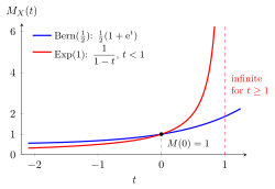
MGFs of a Bernoulli(1/2) and an Exponential(1) variable, both equal to 1 at t = 0; the exponential MGF grows without bound as t approaches 1.

Both curves pass through $(0,1)$ , since $M_X(0)=\mathbb{E}[1]=1$ for every $X$ . The $\operatorname{Bern}(\tfrac{1}{2})$ MGF $\tfrac{1}{2}(1+\mathrm{e}^t)$ is finite for every $t$ , because $X$ takes only the values $0$ and $1$ . The exponential MGF $1/(1-t)$ is finite only for $t<1$ and grows without bound as $t$ approaches $1$ : for $t\ge1$ the factor $\mathrm{e}^{tx}$ outweighs the density $\mathrm{e}^{-x}$ and the integral diverges. It is finite on $(-\infty,1)$ , which contains a neighbourhood of $0$ , and that is all the definition asks for.

Move $t$ along the curve $M_X(t)=\mathbb{E}[\mathrm{e}^{tX}]$ $E [e^{tX}]$ . Every MGF passes through $(0,1)$ ; for $\operatorname{Exp}(\lambda)$ it is finite only for $t<\lambda$ $λ$ .

The parameter $t$ sets the weighting. For $t>0$ $0$ , $\mathrm{e}^{tX}$ gives the largest values of $X$ the most weight, so a heavy right tail makes $M_X(t)$ large or infinite; for $t<0$ the left tail matters. Finiteness at $t=0$ alone says nothing, as $M_X(0)=1$ always. Near $t=0$ $0$ , $\mathrm{e}^{tX}\approx1+tX+t^2X^2/2$ $t^{2} X^{2} /2$ , which is why the derivatives at zero give the moments.

Two further rules make the MGF practical: independent sums multiply MGFs, and equal MGFs near zero mean equal distributions. Together they identify sums such as merged Poisson counts without summing over all the ways in which each total can arise.

Key Results¶

$M_X(0)=1$ $1$ .
Discrete variables use $\displaystyle M_X(t)=\sum_x\mathrm{e}^{tx}p_X(x)$ $x \sum e^{t x} p_{X} (x)$ ; density models use $M_X(t)=\int \mathrm{e}^{tx}f_X(x)\,\mathrm{d}x$ $\int e^{t x} f_{X} (x) d x$ .

Examples¶

For $\operatorname{Bern}(p)$ , $M_X(t)=1-p+p\mathrm{e}^t$ $p e^{t}$ .
For $\operatorname{Exp}(\lambda)$ , $M_X(t)=\lambda/(\lambda-t)$ for $t<\lambda$ $λ$ ; it is infinite for $t\ge\lambda$ $λ$ .

Prerequisites¶

Sources¶

Nicky van Foreest · Probability Distributions · Week 1

Aliases: MGF, m.g.f. Symbols: delta, infinity, integral, lambda, sum

Last updated: 20 October 2026 03:02