Sample Mean¶

Definition¶

For random variables $X_1,\ldots,X_n$ and $n\ge1$ $1$ , their sample mean is

\bar X_n=\frac{1}{n}\sum_{i=1}^nX_i.

The sum adds the $n$ observations before dividing by $n$ . No independence assumption is needed to define this arithmetic average.

Interpretation¶

The sample mean summarizes $n$ observations by their arithmetic average. Before the data are observed, $\bar X_n$ is a random variable with its own expectation, variance and sampling distribution; the observed average $\bar x_n$ is one realized number.

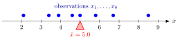
Eight observations marked as dots on a number line from 2 to 9, with a balance point at their mean 5.0.

The figure marks eight observations on a number line. Their mean $\bar x=(2.1+3.4+3.9+4.6+5.0+5.8+6.7+8.5)/8=5.0$ is the balance point: the deviations to the left and right cancel, $\displaystyle \sum_i(x_i-\bar x)=0$ $0$ . A single far-away observation moves the balance point; replacing $8.5$ by $16.5$ raises the mean by $1$ to $6.0$ .

For independent observations with common mean $\mu$ and finite variance $\sigma^2$ , the sample mean has its own distribution: centred at $\mu$ , with variance $\sigma^2/n$ . Raise $n$ to see it narrow.

Two properties make $\bar X_n$ a useful estimate of the population mean $\mu$ . It is centred correctly, $\mathbb{E}\bar X_n=\mu$ $μ$ , which needs only linearity of expectation. With independent observations of common variance $\sigma^2$ , its variance $\sigma^2/n$ shrinks, so the standard deviation $\sigma/\sqrt n$ halves when the sample size is multiplied by four. Without independence the second property can fail: if all $X_i$ equal $X_1$ , then $\bar X_n=X_1$ has variance $\sigma^2$ for every $n$ .

These two properties lead to the weak and strong law of large numbers, which say that $\bar X_n$ approaches $\mu$ , and to the central limit theorem, which describes the shape of the remaining error. A common confusion is between $\bar X_n$ and $\mu$ : the sample mean is computed from data and varies from sample to sample, while $\mu$ is a fixed property of the distribution.

Key Results¶

If every $X_i$ has mean $\mu$ , then $\mathbb{E}\bar X_n=\mu$ without independence.
If the observations are independent with common variance $\sigma^2$ , then $\operatorname{Var}(\bar X_n)=\sigma^2/n$ $σ^{2} / n$ .

Examples¶

For observations $2,4,9$ , the observed sample mean is $(2+4+9)/3=5$ $5$ .
For $100$ i.i.d. $\operatorname{Exp}(2)$ observations, the sample mean has expectation $1/2$ and variance $1/(4\cdot100)=1/400$ $1/400$ .

Further Properties¶

For realized observations $x_1,\ldots,x_n$ , the observed average is $\displaystyle \bar x_n=n^{-1}\sum_i x_i$ $n^{- 1} i \sum x_{i}$ . A sample proportion is the sample mean of success indicators.

Prerequisites¶

Expectation

Sources¶

Probability Distributions · supporting concept

Aliases: sample average, empirical mean, X bar Symbols: mu, sigma, square root, sum

Last updated: 20 October 2026 03:02