Moment¶

Definition¶

Let $X$ be a random variable and let $r\ge1$ be a natural number. If $\mathbb{E}|X|^r<\infty$ $\infty$ , the $r$ th moment (or raw moment, moment about the origin) of $X$ is

\mathbb{E}[X^r].

Writing $\mu=\mathbb{E}X$ for the first moment, the $r$ th central moment (moment about the mean) is

\mathbb{E}[(X-\mu)^r].

If $\mathbb{E}|X|^r=\infty$ $\infty$ , the $r$ th moment does not exist. Both moments are expectations of a function of $X$ , so by LOTUS they are computed from the PMF as $\displaystyle \sum_x x^r p_X(x)$ or from the PDF as $\int x^r f_X(x)\,\mathrm{d}x$ , and similarly with $(x-\mu)^r$ $μ)^{r}$ .

Interpretation¶

Moments summarize a distribution through averages of powers. Raw moments are measured from $0$ ; central moments are measured from the mean, so they describe the shape of the distribution around its centre and do not change when $X$ is shifted. Higher powers give large deviations more weight, so higher moments are increasingly sensitive to the tails.

For $X$ taking the values $1,2,3$ with probabilities $0.5,0.3,0.2$ :

raw moments: $\mathbb{E}X=1.7$ $1.7$ , $\mathbb{E}[X^2]=0.5+1.2+1.8=3.5$ and $\mathbb{E}[X^3]=0.5+2.4+5.4=8.3$ $8.3$ ;
central moments: the deviations from $\mu=1.7$ are $-0.7,0.3,1.3$ , so the second central moment is $0.5(0.49)+0.3(0.09)+0.2(1.69)=0.61$ and the third is $0.5(-0.343)+0.3(0.027)+0.2(2.197)=0.276$ $0.276$ .

Probability bars at 1, 2 and 3 with masses 0.5, 0.3 and 0.2, used to compute the first three moments.

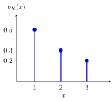
The positive third central moment reflects the long right tail: the single large deviation $1.3$ outweighs the more likely deviation $-0.7$ once it is cubed.

Choose the order $r$ and measure from $0$ or from $\mu$ . Each lower bar is one contribution $x^r p_X(x)$ or $(x-\mu)^r p_X(x)$ $μ)^{r} p_{X} (x)$ , and the moment is their sum. Shift every value to see that only the raw moments change.

The order of operations matters. The second moment $\mathbb{E}[X^2]$ averages the squares, whereas $(\mathbb{E}X)^2$ squares the average; here $3.5$ against $1.7^2=2.89$ $2.89$ . Their difference is the second central moment, $3.5-2.89=0.61$ $0.61$ .

Key Results¶

The first moment is the expectation, and the first central moment is always $0$ . The second central moment is the variance; expanding the power and using linearity of expectation expresses central moments through raw moments:

\begin{aligned} \operatorname{Var}(X)&=\mathbb{E}[(X-\mu)^2]\\ &=\mathbb{E}[X^2]-\mu^2,\\ \mathbb{E}[(X-\mu)^3]&=\mathbb{E}[X^3]-3\mu\,\mathbb{E}[X^2] +2\mu^3. \end{aligned}

The cross terms do not cancel: the third central moment is not $\mathbb{E}[X^3]-\mu^3$ $μ^{3}$ . When the third moment exists and the standard deviation satisfies $\sigma>0$ $0$ , the third central moment divided by $\sigma^3$ is the skewness, a measure of asymmetry. This standardized coefficient is undefined for a constant random variable, for which $\sigma=0$ $0$ .

Since a variance is never negative, $\mathbb{E}[X^2]\ge(\mathbb{E}X)^2$ $(E X)^{2}$ , with equality exactly when $X$ is constant almost surely.
For constants $a,b$ , the $r$ th central moment of $a+bX$ is $b^r$ (not $|b|^r$ ) times that of $X$ . In particular, shifting by $a$ leaves all central moments unchanged, and the odd central moments change sign when $b=-1$ $- 1$ . Raw moments are not shift-invariant: $\mathbb{E}[(a+bX)^2]=a^2+2ab\,\mathbb{E}X+b^2\,\mathbb{E}[X^2]$ $b^{2} E [X^{2}]$ .
If the $s$ th moment exists, so does every $r$ th moment with $r\le s$ $s$ , because $|x|^r\le1+|x|^s$ $∣ x ∣^{s}$ . The converse fails: moments can fail to exist for heavy-tailed distributions even when lower moments are finite.
If $X$ is bounded, say $|X|\le c$ $c$ , every moment exists and $|\mathbb{E}[X^r]|\le c^r$ $c^{r}$ .
For an indicator random variable $I_A$ , $I_A^r=I_A$ $I_{A}$ , so every moment equals $\mathbb{P}(A)$ .
If the moment generating function is finite on an open interval around $0$ , all moments exist and $\mathbb{E}[X^n]=M_X^{(n)}(0)$ (moments from the MGF).

Examples¶

For a fair die, $\mathbb{E}X=21/6=3.5$ and $\mathbb{E}[X^2]=(1+4+9+16+25+36)/6=91/6$ $91/6$ , so $\operatorname{Var}(X)=91/6-49/4=35/12$ $35/12$ .
For $X\sim\operatorname{Bern}(p)$ (Bernoulli distribution), $X^r=X$ $X$ , so $\mathbb{E}[X^r]=p$ for every $r$ and $\operatorname{Var}(X)=p-p^2=p(1-p)$ $p)$ .
For $X\sim\operatorname{Unif}(0,1)$ $Unif (0, 1)$ , $\mathbb{E}[X^r]=\int_0^1 x^r\,\mathrm{d}x=1/(r+1)$ $1)$ , so $\operatorname{Var}(X)=1/3-1/4=1/12$ $1/12$ .
For $X\sim\operatorname{Exp}(\lambda)$ $Exp (λ)$ , $\mathbb{E}[X^n]=n!/\lambda^n$ $n! / λ^{n}$ ; the second central moment is $2/\lambda^2-1/\lambda^2=1/\lambda^2$ $1/ λ^{2}$ .
For the three-point $X$ above and $Y=2X+1$ $1$ , $\mathbb{E}Y=2(1.7)+1=4.4$ $4.4$ , the second central moment of $Y$ is $2^2(0.61)=2.44$ and the third is $2^3(0.276)=2.208$ $2.208$ .
If $X$ has a symmetric distribution about its mean, every odd central moment that exists is $0$ : the deviations $X-\mu$ and $\mu-X$ have the same distribution.
The density $f(x)=2x^{-3}$ for $x\ge1$ has finite mean $\mathbb{E}X=\int_1^\infty 2x^{-2}\,\mathrm{d}x=2$ $2$ , but $\mathbb{E}[X^2]=\int_1^\infty 2x^{-1}\,\mathrm{d}x=\infty$ $\infty$ , so its variance does not exist.

Prerequisites¶

Sources¶

Nicky van Foreest · Probability Distributions · Week 1

Aliases: raw moment, moment about the origin, central moment, moment about the mean Keywords: nth moment, first moment, second moment, nth central moment, E[X^r], existence of moments Symbols: infinity, integral, lambda, mu, sigma, sum

Last updated: 27 October 2026 11:52