Normal Approximation to the Binomial¶

Approximation¶

For $X_n\sim\operatorname{Bin}(n,p)$ with fixed $p\in(0,1)$ $(0, 1)$ , as $n\to\infty$ $\infty$ ,

\begin{aligned} \frac{X_n-np}{\sqrt{np(1-p)}}\xrightarrow{d}\mathcal{N}(0,1). \end{aligned}

For a finite $n$ the normal approximation can be inaccurate when $np$ or $n(1-p)$ is small; there is no universal finite- $n$ accuracy guarantee.

A Binomial Distribution count is a sum of i.i.d. Bernoulli indicators. The Central Limit Theorem applied to that sum gives the stated normal limit after centring and scaling.

Interpretation¶

A binomial count with many trials is approximately normal with the same mean $np$ and variance $np(1-p)$ $p)$ . The reason is that $\operatorname{Bin}(n,p)$ is the distribution of a sum of $n$ i.i.d. Bernoulli indicators, so the central limit theorem applies to it.

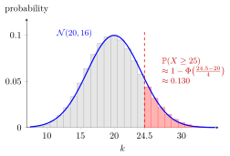
Binomial(100, 0.2) probability bars with the normal density of mean 20 and variance 16 overlaid; the bars from 25 upwards are highlighted and the normal tail is taken from 24.5.

The figure compares $X\sim\operatorname{Bin}(100,0.2)$ with $\mathcal{N}(20,16)$ : mean $np=20$ $20$ , variance $np(1-p)=16$ $16$ , standard deviation $4$ . The highlighted tail has exact probability $\mathbb{P}(X\ge25)\approx0.131$ $0.131$ . With the continuity correction, the normal tail from $24.5$ gives $1-\Phi(1.125)\approx0.130$ $0.130$ , while starting at $25$ would give $1-\Phi(1.25)\approx0.106$ $0.106$ .

Change $n$ and $p$ : once $np(1-p)$ is large the bars follow the normal density with mean $np$ and variance $np(1-p)$ $p)$ .

The limit statement keeps $p$ fixed while $n$ grows. For a finite $n$ , the approximation is poor when $np$ or $n(1-p)$ is small: the binomial is then skewed and piled up near $0$ or $n$ , while the normal curve is symmetric and puts probability below $0$ or above $n$ . Standardizing the count gives the displayed form; dividing it by $n$ instead gives the proportion of successes $X/n$ , a sample mean of indicators, which is approximately $\mathcal{N}(p,p(1-p)/n)$ $p) / n)$ .

A common slip is to use $np$ as the variance, or to forget the square root in the standard deviation $\sqrt{np(1-p)}$ . In the figure the standard deviation is $4$ , not $16$ or $20$ .

Key Results¶

For fixed $0<p<1$ $1$ , $X_n\sim\operatorname{Bin}(n,p)$ has $\mathbb{E}X_n=np$ and $\operatorname{Var}(X_n)=np(1-p)$ $p)$ .
For a finite- $n$ threshold $k$ , a continuity-corrected approximation is $\mathbb{P}(X_n\le k)\approx\Phi((k+1/2-np)/\sqrt{np(1-p)})$ $n p) / n p (1 - p))$ .

Examples¶

For $X\sim\operatorname{Bin}(100,0.5)$ $Bin (100, 0.5)$ , $\mathbb{P}(X\le60)\approx\Phi(2.1)\approx0.9821$ $0.9821$ .
For $X\sim\operatorname{Bin}(100,0.2)$ $Bin (100, 0.2)$ , $\mathbb{P}(X\ge25)\approx1-\Phi((24.5-20)/4)\approx0.1303$ $0.1303$ .

Prerequisites¶

Sources¶

Nicky van Foreest · Probability Distributions · Week 8

Aliases: de Moivre-Laplace theorem Symbols: element of, infinity, phi, square root

Last updated: 20 October 2026 03:02