Adam’s Law: Total Expectation¶

Theorem¶

For random variables $X$ and $Y$ with $\mathbb{E}|Y|<\infty$ $\infty$ ,

\begin{aligned} \mathbb{E}[\mathbb{E}[Y\mid X]]=\mathbb{E}[Y]. \end{aligned}

Interpretation¶

Adam’s law computes a mean in two steps: first the mean of $Y$ within each scenario $X=x$ $x$ , then the average of these conditional means over the distribution of $X$ . Averaging the conditional average recovers the original average.

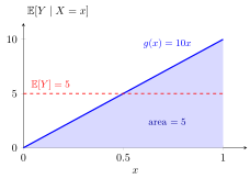
Graph of the conditional mean 10x of Y given X = x for x from 0 to 1, with the shaded area under it equal to 5 and a horizontal line at the overall mean E(Y) = 5.

For $X\sim\operatorname{Unif}(0,1)$ and $Y\mid X\sim\operatorname{Bin}(10,X)$ $Bin (10, X)$ , the conditional mean is $g(x)=10x$ $10 x$ . Since $X$ has density $1$ on $(0,1)$ , the average of $g(X)$ is the shaded area under the line, $\int_0^1 10x\,\mathrm{d}x=5$ $5$ , which is the height of the dashed line $\mathbb{E}[Y]=5$ $5$ .

Here $X$ is discrete with three values. $\mathbb{E}[Y\mid X=x]$ is the centre of each group; averaging these with the probabilities $\mathbb{P}(X=x)$ gives $\mathbb{E}Y$ .

The inner expectation $\mathbb{E}[Y\mid X]=g(X)$ is a random variable; the outer one averages it with the distribution of $X$ , by LOTUS: a sum over $p_X(x)$ for discrete $X$ , an integral against $f_X(x)$ for continuous $X$ . The condition $\mathbb{E}|Y|<\infty$ makes both sides finite and well defined. The method pays off in two-stage models, where the conditional law of $Y$ is simple but its unconditional law is not.

For a discrete $X$ the law is the law of total expectation over a partition with the cases $\{X=x\}$ $x}$ , and taking $Y$ an indicator gives back the law of total probability, discrete or continuous. The corresponding rule for variances returns later as Eve’s law.

The outer average must use the distribution of $X$ : if $X$ had density $2x$ on $(0,1)$ instead, the same conditional means $10x$ would give $\mathbb{E}Y=\int_0^1 10x\cdot2x\,\mathrm{d}x=20/3$ $20/3$ , not $5$ .

Key Results¶

For discrete $X$ , $\displaystyle \mathbb{E}Y=\sum_x\mathbb{E}[Y\mid X=x]p_X(x)$ $x] p_{X} (x)$ ; for density $X$ , use the corresponding integral.
Conditioning on more information first and then on less gives the conditional expectation given the smaller information: $\mathbb{E}[\mathbb{E}[Y\mid X,Z]\mid Z]=\mathbb{E}[Y\mid Z]$ (Adam's law with extra conditioning).

Examples¶

If $X\sim\operatorname{Unif}(0,1)$ and $Y\mid X\sim\operatorname{Bin}(10,X)$ $Bin (10, X)$ , then $\mathbb{E}Y=\mathbb{E}[10X]=5$ $5$ .
If $X\sim\operatorname{Exp}(2)$ and $Y\mid X\sim\operatorname{Pois}(X)$ $Pois (X)$ , then $\mathbb{E}Y=\mathbb{E}X=1/2$ $1/2$ .

Prerequisites¶

Conditional Expectation Given a Random Variable

Sources¶

Nicky van Foreest · Probability Distributions · Week 4

Aliases: law of total expectation, total expectation formula, law of iterated expectations, tower property, law of double expectation Symbols: infinity, integral, sum

Last updated: 20 October 2026 03:02