Conditional Probability Mass Function¶

Definition¶

For discrete random variables $X$ and $Y$ and a value $y$ with $p_Y(y)>0$ $0$ , the conditional PMF of $X$ given $Y=y$ is

\begin{aligned} p_{X\mid Y}(x\mid y)=\frac{p_{X,Y}(x,y)}{p_Y(y)}, \quad p_Y(y)>0. \end{aligned}

The numerator is the Joint Probability Mass Function, and the denominator is its Marginal Probability Mass Function for $Y$ . This is the ordinary Conditional Probability rule applied to $\{X=x\}$ and $\{Y=y\}$ when the latter has positive probability.

Interpretation¶

A conditional PMF rescales the part of a joint table consistent with the observed discrete value. Once $Y=y$ is known, only the pairs with that value of $y$ remain possible, and their masses are divided by $p_Y(y)$ so that they again add up to $1$ , just as in conditional probability for events.

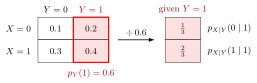
A 2 by 2 joint probability table with the column Y = 1 boxed, its sum 0.6 marked, and an arrow to the rescaled column 1/3 and 2/3, the conditional PMF of X given Y = 1.

In the diagram the column $Y=1$ holds the masses $0.2$ and $0.4$ , with total $p_Y(1)=0.6$ $0.6$ . Dividing by $0.6$ gives $p_{X\mid Y}(0\mid1)=\tfrac{1}{3}$ and $p_{X\mid Y}(1\mid1)=\tfrac{2}{3}$ $\frac{2}{3}$ . Unconditionally $\mathbb{P}(X=1)=0.3+0.4=0.7$ $0.7$ , so learning $Y=1$ lowers the probability of $X=1$ slightly.

Here $y$ runs up the vertical axis. Fix $Y=y$ $y$ : keep that row of masses and divide by $p_Y(y)$ so that they sum to $1$ .

For each fixed $y$ with $p_Y(y)>0$ $0$ , $x\mapsto p_{X\mid Y}(x\mid y)$ is an ordinary PMF: nonnegative and summing to $1$ . Dividing by one number keeps the relative sizes of the masses, so the conditional PMF has the shape of the selected column. As a function of $y$ for fixed $x$ it is not a PMF: in the table, $p_{X\mid Y}(1\mid0)+p_{X\mid Y}(1\mid1)=0.75+\tfrac{2}{3}\neq1$ $1$ . When $p_Y(y)=0$ the conditional PMF is not defined.

Independence of $X$ and $Y$ means that every conditional PMF equals the marginal $p_X$ : observing $Y$ changes nothing. Multiplying back, $p_{X,Y}(x,y)=p_{X\mid Y}(x\mid y)p_Y(y)$ $y) p_{Y} (y)$ , which is how two-stage models are built, as in the chicken–egg theorem, where $N$ is Poisson and the count given $N=n$ is binomial. Summing over $y$ gives the law of total probability in PMF form, $\displaystyle p_X(x)=\sum_yp_{X\mid Y}(x\mid y)p_Y(y)$ $y) p_{Y} (y)$ .

Key Results¶

For $p_Y(y)>0$ $0$ , $\displaystyle \sum_xp_{X\mid Y}(x\mid y)=1$ $1$ .
$p_{X,Y}(x,y)=p_{X\mid Y}(x\mid y)p_Y(y)$ $y) p_{Y} (y)$ .

Examples¶

For the table $0.1,0.2,0.3,0.4$ at $(0,0),(0,1),(1,0),(1,1)$ , $\mathbb{P}(X=1\mid Y=1)=0.4/0.6=2/3$ $2/3$ .
If $X=Y\sim\operatorname{Bern}(1/2)$ $Bern (1/2)$ , then $\mathbb{P}(X=1\mid Y=1)=1$ $1$ .

Prerequisites¶

Sources¶

Nicky van Foreest · Probability Distributions · Week 1

Aliases: conditional PMF, conditional mass function Symbols: sum

Last updated: 20 October 2026 03:02