Conditional Density Given an Event¶

Definition¶

Let $Y$ be a continuous random variable and $A$ an event with $\mathbb{P}(A)>0$ $0$ . The conditional CDF of $Y$ given $A$ is

\begin{aligned} F_{Y\mid A}(y)=\mathbb{P}(Y\leq y\mid A). \end{aligned}

Where the derivative exists, the conditional density of $Y$ given $A$ is

\begin{aligned} f_{Y\mid A}(y)=\frac{\mathrm{d}}{\mathrm{d}y}F_{Y\mid A}(y). \end{aligned}

Equivalently, by Bayes' rule,

\begin{aligned} f_{Y\mid A}(y)=\frac{\mathbb{P}(A\mid Y=y)f_Y(y)}{\mathbb{P}(A)}. \end{aligned}

Here $\mathbb{P}(A\mid Y=y)$ is the conditional probability given the value $y$ , determined except possibly on a set of values $y$ of probability zero, where it may be chosen arbitrarily; it is not an elementary ratio, whose denominator $\mathbb{P}(Y=y)$ would be zero.

Interpretation¶

Conditioning on an event $A$ reweights the original density of $Y$ by how compatible each value $y$ is with $A$ , and then divides by $\mathbb{P}(A)$ so that the total area is again $1$ .

An exponential density with the region y greater than 1 shaded, and the conditional density given that event: the same curve restricted to y greater than 1 and scaled up by 1 over P(A).

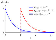
In the illustrated example, $Y\sim\operatorname{Exp}(2)$ and $A=\{Y>1\}$ $1}$ , with $\mathbb{P}(A)=\mathrm{e}^{-2}\approx0.14$ $0.14$ . Keep the shaded part of the density on $A$ and divide by $\mathbb{P}(A)$ : $f_{Y\mid A}(y)=2\mathrm{e}^{-2y}/\mathrm{e}^{-2}=2\mathrm{e}^{-2(y-1)}$ for $y>1$ and $0$ elsewhere. The red curve is the original density shifted one unit to the right, the memoryless property.

Move $c$ : on $A=\{Y>c\}$ the density is divided by $\mathbb{P}(A)$ , and outside $A$ it is $0$ . For $\operatorname{Exp}(2)$ the result is the same density shifted to start at $c$ .

The Bayes form of the definition covers two kinds of event. If $A=\{Y\in B\}$ is decided by $Y$ itself, then $\mathbb{P}(A\mid Y=y)$ is $1$ on $B$ and $0$ outside it, and conditioning simply cuts the density to $B$ and rescales it. If $A$ also depends on other randomness, $\mathbb{P}(A\mid Y=y)$ lies between $0$ and $1$ and the density is reweighted smoothly. For example, let $Y\sim\operatorname{Unif}(0,1)$ and let $A$ be the event that a coin with success probability $Y$ shows heads; then $\mathbb{P}(A\mid Y=y)=y$ $y$ , $\mathbb{P}(A)=1/2$ and $f_{Y\mid A}(y)=2y$ on $(0,1)$ .

With this density, the conditional expectation given an event from Probability Theory is $\mathbb{E}[Y\mid A]=\int y\,f_{Y\mid A}(y)\,\mathrm{d}y$ $\int y f_{Y ∣ A} (y) d y$ ; in the figure it equals $1+1/2=3/2$ $3/2$ . Conditioning on the value of another variable, which has probability zero, needs the conditional PDF instead.

Cutting without rescaling is a common slip: the cut density $2\mathrm{e}^{-2y}$ on $y>1$ integrates to $\mathrm{e}^{-2}$ , not $1$ .

Key Results¶

If $A=\{Y\in B\}$ $B}$ , then $f_{Y\mid A}(y)=\indicator_{B}(y)f_Y(y)/\mathbb{P}(Y\in B)$ except possibly on a set of zero length.
The conditional density $f_{Y\mid A}$ integrates to one whenever $\mathbb{P}(A)>0$ $0$ .

Examples¶

For $Y\sim\operatorname{Unif}(0,1)$ and $A=\{Y>1/2\}$ $1/2}$ , the conditional density is $2$ on $(1/2,1)$ .
For $Y\sim\operatorname{Exp}(2)$ and $A=\{Y>1\}$ $1}$ , the conditional density is $2\mathrm{e}^{-2(y-1)}$ for $y>1$ $1$ .

Prerequisites¶

Sources¶

Nicky van Foreest · Probability Distributions · Week 4

Symbols: element of, integral

Last updated: 20 October 2026 03:02