Bayes and Total Probability: Four Forms¶

Theorem¶

Write $m_X,m_Y$ for marginal mass or density functions and $m_{X\mid Y},m_{Y\mid X}$ for the corresponding conditional functions. Where the denominator is positive and finite,

m_{X\mid Y}(x\mid y)=\frac{m_{Y\mid X}(y\mid x)m_X(x)}{m_Y(y)}.

The four total-probability forms are:

$X$	$Y$	Marginalization over $Y$
Discrete	Discrete	$\displaystyle p_X(x)=\sum_y p_{X\mid Y}(x\mid y)p_Y(y)$
Continuous	Continuous	$f_X(x)=\int f_{X\mid Y}(x\mid y)f_Y(y)\,\mathrm{d}y$
Discrete	Continuous	$p_X(x)=\int p_{X\mid Y}(x\mid y)f_Y(y)\,\mathrm{d}y$
Continuous	Discrete	$\displaystyle f_X(x)=\sum_y f_{X\mid Y}(x\mid y)p_Y(y)$

Use appropriate conditional mass or density versions; continuity of marginals alone does not establish a joint density.

For discrete conditional laws use a Conditional Probability Mass Function; for conditional laws with densities use a Conditional Probability Density Function. Both express Conditional Probability, but density conditioning at a point is not division by the probability of that point.

Interpretation¶

The same factorization works whether each variable is discrete or continuous: sum over discrete values and integrate over continuous ones. In every case "joint $=$ conditional $\times$ marginal" produces both Bayes' rule and the law of total probability, with $m$ standing for a PMF or a density as the type of each variable requires.

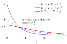
Two conditional densities of Y given H = 0 and H = 1, and the posterior probability that H = 1 as a decreasing curve that passes 1/2 at y = ln 2, where the two densities are equal.

In this example, $H\sim\operatorname{Bern}(\tfrac{1}{2})$ is discrete, while $Y$ has conditional densities $f_{Y\mid H}(y\mid0)=\mathrm{e}^{-y}$ and $f_{Y\mid H}(y\mid1)=2\mathrm{e}^{-2y}$ for $y>0$ $0$ . Summing over $H$ gives $f_Y(y)=\tfrac{1}{2}\mathrm{e}^{-y}+\tfrac{1}{2}\cdot2\mathrm{e}^{-2y}$ $2 e^{- 2 y}$ , and Bayes' rule gives $\mathbb{P}(H=1\mid Y=y)=2/(\mathrm{e}^y+2)$ $2)$ , the red curve. It starts at $\tfrac{2}{3}$ for $y$ near $0$ and decreases; at $y=\ln2$ $ln 2$ , where the two densities are equal, the posterior equals the prior $\tfrac{1}{2}$ . Small observations favour $H=1$ $1$ , whose density puts more weight near $0$ .

To read the table, note that the variable summed or integrated out is $Y$ , so the operation follows the type of $Y$ . The left-hand side follows the type of $X$ : a PMF $p_X$ if $X$ is discrete, a density $f_X$ if $X$ is continuous. In the mixed forms a probability and a density appear in one formula. Heuristically, $f_Y(y)$ stands for $\mathbb{P}(y<Y\le y+h)/h$ for a small $h>0$ $0$ , and the width $h$ cancels between numerator and denominator.

All four forms extend the law of total probability and Bayes' rule for events. The purely continuous forms are treated separately in the continuous law of total probability and the continuous Bayes rule.

Key Results¶

When $X$ is discrete and $Y$ continuous, $p_{X\mid Y}(x\mid y)=f_{Y\mid X}(y\mid x)p_X(x)/f_Y(y)$ and $\displaystyle f_Y(y)=\sum_xf_{Y\mid X}(y\mid x)p_X(x)$ $x) p_{X} (x)$ .
When $X$ is continuous and $Y$ discrete, $f_{X\mid Y}(x\mid y)=p_{Y\mid X}(y\mid x)f_X(x)/p_Y(y)$ and $p_Y(y)=\int p_{Y\mid X}(y\mid x)f_X(x)\,\mathrm{d}x$ $x) f_{X} (x) d x$ .

Examples¶

If $Y\sim\operatorname{Unif}(0,1)$ and $X\mid Y=y\sim\operatorname{Bern}(y)$ $Bern (y)$ , then $f_{Y\mid X}(y\mid1)=2y$ on $(0,1)$ .
If $H\sim\operatorname{Bern}(1/2)$ $Bern (1/2)$ , $Y\mid H=0\sim\operatorname{Exp}(1)$ $Exp (1)$ , and $Y\mid H=1\sim\operatorname{Exp}(2)$ $Exp (2)$ , then $\mathbb{P}(H=1\mid Y=y)=2\mathrm{e}^{-2y}/(\mathrm{e}^{-y}+2\mathrm{e}^{-2y})$ for $y>0$ $0$ .

Prerequisites¶

Sources¶

Nicky van Foreest · Probability Distributions · Week 2

Symbols: integral, sum

Last updated: 20 October 2026 03:02