Continuous Law of Total Probability¶

Theorem¶

For continuous random variables $X$ and $Y$ for which the conditional density $f_{X\mid Y}$ exists,

\begin{aligned} f_X(x)=\int f_{X\mid Y}(x\mid y)\,f_Y(y)\,\mathrm{d}y \end{aligned}

for every $x$ except possibly on a set of zero length, for example at finitely many points.

The left side is the Marginal Probability Density Function of the response. It is recovered by averaging the conditional densities over the other variable’s marginal law.

Interpretation¶

The continuous law of total probability describes a two-stage model: first $Y$ is drawn, then $X$ is drawn from the conditional density $f_{X\mid Y}(\cdot\mid y)$ $y)$ . The unconditional density of $X$ is then a weighted mixture of the conditional densities, with the density of $Y$ as the weight.

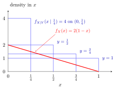
Uniform conditional densities of X given Y = 1/4, 1/2, 3/4 and 1, drawn as rectangles of decreasing height, and the mixed marginal density 2(1 - x) obtained by averaging them.

For $X\mid Y=y\sim\operatorname{Unif}(0,y)$ $Unif (0, y)$ , each conditional density is a rectangle of height $1/y$ on $(0,y)$ : heights $4$ , $2$ , $4/3$ and $1$ for $y=1/4,1/2,3/4,1$ $1/4, 1/2, 3/4, 1$ . A point $x$ lies under the rectangles with $y>x$ only, so with $f_Y(y)=2y$ on $(0,1)$ the average is $f_X(x)=\int_x^1(1/y)2y\,\mathrm{d}y=2(1-x)$ for $0<x<1$ $1$ . Values near $1$ lie under few rectangles, so the red marginal decreases.

Cut the range of $Y$ into $m$ slices: each contributes $f_{X\mid Y}(x\mid y_j)f_Y(y_j)\Delta y$ $y_{j}) f_{Y} (y_{j}) Δ y$ . Raise $m$ and the sum becomes $f_X$ .

The formula is the law of total probability $\displaystyle \mathbb{P}(A)=\sum_i\mathbb{P}(A\mid B_i)\mathbb{P}(B_i)$ with the cases $B_i$ replaced by the values $y$ , the sum by an integral and $\mathbb{P}(B_i)$ by $f_Y(y)\,\mathrm{d}y$ ; the slider above shows exactly this limit of sums. Since $f_{X\mid Y}(x\mid y)f_Y(y)=f_{X,Y}(x,y)$ $f_{X, Y} (x, y)$ , it is also the computation of a marginal density from the joint density.

The same integral is the normalizing denominator in the continuous Bayes rule, and the same averaging applied to means returns as Adam’s law.

The integration range is easy to get wrong: $f_{X\mid Y}(x\mid y)$ is zero unless $y>x$ $x$ , so the integral runs from $x$ to $1$ . Integrating over all of $(0,1)$ would give the constant $2$ , which integrates to $2$ rather than $1$ ; checking that the result integrates to one catches such errors.

Key Results¶

The event form is $\mathbb{P}(X\in A)=\int\mathbb{P}(X\in A\mid Y=y)f_Y(y)\,\mathrm{d}y$ $y) f_{Y} (y) d y$ .
Integrating the conditional density mixture over $x$ gives total probability one.

Examples¶

For density $2$ on $0<x<y<1$ $1$ , $f_X(x)=\int_x^1(1/y)(2y)\,\mathrm{d}y=2(1-x)$ for $0<x<1$ $1$ .
If $Y\sim\operatorname{Unif}(0,1)$ and $X\mid Y=y\sim\operatorname{Bern}(y)$ $Bern (y)$ , then $\mathbb{P}(X=1)=\int_0^1y\,\mathrm{d}y=1/2$ $1/2$ , using the event form.

Prerequisites¶

Sources¶

Nicky van Foreest · Probability Distributions · Week 2

Aliases: continuous LOTP Symbols: delta, element of, integral, sum

Last updated: 20 October 2026 03:02