Chicken–Egg Theorem¶

Theorem¶

Let $\lambda>0$ $0$ , $0<p<1$ and $q=1-p$ $p$ . If $N\sim\operatorname{Pois}(\lambda)$ and, given $N=n$ $n$ , $X\sim\operatorname{Bin}(n,p)$ for every $n\ge0$ $0$ , then $X\sim\operatorname{Pois}(\lambda p)$ and $N-X\sim\operatorname{Pois}(\lambda q)$ $Pois (λ q)$ , and $X$ and $N-X$ are independent.

The Poisson Distribution supplies the random total $N$ . Given that total, the Conditional Probability Mass Function of $X$ is a Binomial Distribution PMF: independently labelling $n$ items produces a binomial count before averaging over $N$ .

Interpretation¶

A Poisson total divided by binomial labelling produces two independent Poisson counts, even though their sum is the original total. The name comes from the picture in the figure: a Poisson number of eggs is laid, and each egg hatches independently with probability $p$ .

A row of ten eggs, a Poisson number of them, split by independent hatching into three that hatch and seven that do not, illustrating two independent Poisson counts.

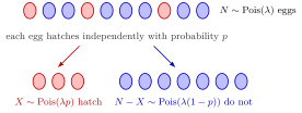
In the sample shown, ten eggs are laid; three hatch (red) and seven do not (blue). Over repeated samples the hatched count is $\operatorname{Pois}(\lambda p)$ , the unhatched count is $\operatorname{Pois}(\lambda q)$ , and the two counts are independent: for instance, $\lambda=10$ and $p=0.3$ give $\operatorname{Pois}(3)$ and $\operatorname{Pois}(7)$ .

$N\sim\operatorname{Pois}(\lambda)$ eggs each hatch with probability $p$ . The hatched and unhatched counts are independent Poisson variables.

The surprise is the independence. For a fixed total $n\ge1$ the counts are dependent, since they must add up to $n$ : many hatched eggs force few unhatched ones. Given $N=0$ $0$ , both counts are constant zero and are independent. With a Poisson total this dependence disappears, because the joint PMF factorizes:

\mathbb{P}(X=k,\,N-X=m) =\mathrm{e}^{-\lambda p}\frac{(\lambda p)^k}{k!}\cdot\mathrm{e}^{-\lambda q}\frac{(\lambda q)^m}{m!}.

This follows from $\mathbb{P}(N=k+m)\binom{k+m}{k}p^kq^m$ by writing $\mathrm{e}^{-\lambda}=\mathrm{e}^{-\lambda p}\mathrm{e}^{-\lambda q}$ and $\lambda^{k+m}=\lambda^k\lambda^m$ $λ^{k} λ^{m}$ ; the factorials $(k+m)!$ cancel. The Poisson assumption on $N$ is what makes the exponential factor split in this way; for other distributions of the total the counts are in general dependent.

The theorem is the basis of Poisson splitting into labelled categories. Read in the other direction, it matches Poisson merging: two independent Poisson counts add up to a Poisson total, and given that total, the first count is binomial.

Key Results¶

If $Y=N-X$ $X$ , then $X\sim\operatorname{Pois}(\lambda p)$ and $Y\sim\operatorname{Pois}(\lambda(1-p))$ independently.
Given $N=n\ge1$ $1$ , the two counts are dependent: they add to $n$ , so $X=k$ forces $Y=n-k$ $k$ . Given $N=0$ $0$ , both are constant zero.

Examples¶

If $N\sim\operatorname{Pois}(10)$ and $p=0.3$ $0.3$ , then $X\sim\operatorname{Pois}(3)$ and $Y\sim\operatorname{Pois}(7)$ independently.
With $\lambda=4$ $4$ , $p=1/2$ $1/2$ , $\mathbb{P}(X=0,Y=0)=\mathrm{e}^{-2}\mathrm{e}^{-2}=\mathrm{e}^{-4}$ $e^{- 4}$ .

Prerequisites¶

Poisson Merging

Sources¶

Nicky van Foreest · Probability Distributions · Week 1

Symbols: lambda

Last updated: 27 October 2026 11:52