Conditioning Trick for Variance¶

Method¶

When $Y$ has a natural conditional structure, for example $Y\mid X=x\sim\operatorname{Pois}(x)$$\mathrm{Pois}(x)$, compute $\operatorname{Var}(Y)$ by decomposing it with Eve's law (total variance). This is a calculation method rather than a separate theorem; it needs $\mathbb{E}[Y^2]<\infty$$\infty$.

Interpretation¶

When the distribution of $Y$ is awkward but $Y$ becomes simple once another variable $X$ is known, compute its mean and variance in two layers: first for fixed $X$, then over $X$, combined by total variance. This avoids finding the marginal distribution of $Y$.

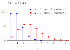
The figure shows the two cases of the first Example: $X$ equals $1$ or $3$ with probability $\tfrac{1}{2}$ each, and $Y\mid X\sim\operatorname{Pois}(X)$$\mathrm{Pois}(X)$. The average conditional variance, the spread within each bar chart, is $(1+3)/2=2$$2$. The variance of the conditional means $1$ and $3$, the spread between the charts, is $1$. The total variance is therefore $\operatorname{Var}(Y)=2+1=3$$3$.

The method has three steps. Name the variable $X$ that makes $Y$ simple; write down $m(X)=\mathbb{E}[Y\mid X]$ and $v(X)=\operatorname{Var}(Y\mid X)$$X)$, here the Poisson mean and variance; then compute $\mathbb{E}[v(X)]$ and $\operatorname{Var}(m(X))$ from the distribution of $X$ alone. The last step needs only the mean and variance of $X$, which is why the Key Result $\operatorname{Var}(Y)=\mathbb{E}X+\operatorname{Var}(X)$ holds for every $X$ with finite second moment. The mean is the same calculation with Adam's law.

The second term is easy to forget. Here $\operatorname{Var}(Y)=3$ exceeds $\mathbb{E}Y=2$$2$, although every conditional Poisson law has variance equal to its mean: the randomness of the rate adds variance. This idea returns later in insurance, where a Poisson claim count with a random rate explains claim counts whose variance exceeds their mean (overdispersion).

Key Results¶

• Compute $m(X)=\mathbb{E}[Y\mid X]$ and $v(X)=\operatorname{Var}(Y\mid X)$ first; then $\operatorname{Var}(Y)=\mathbb{E}[v(X)]+\operatorname{Var}(m(X))$$\mathrm{Var}(m(X))$.
• For $Y\mid X\sim\operatorname{Pois}(X)$ with finite second moment of $X$, $\mathbb{E}Y=\mathbb{E}X$ and $\operatorname{Var}(Y)=\mathbb{E}X+\operatorname{Var}(X)$$\mathrm{Var}(X)$.

Examples¶

• If $X$ is equally likely to be $1$ or $3$ and $Y\mid X\sim\operatorname{Pois}(X)$$\mathrm{Pois}(X)$, then $\mathbb{E}Y=2$ and $\operatorname{Var}(Y)=2+1=3$$3$.
• If $X\sim\operatorname{Bern}(1/2)$ and $Y\mid X\sim\operatorname{Bin}(4,0.2+0.6X)$$0.6X)$, the within variance is $0.64$, the conditional-mean variance is $1.44$, and total variance is $2.08$.

Prerequisites¶

• Eve’s Law: Total Variance

Related Concepts¶

• Poisson Distribution
• Adam’s Law: Total Expectation
• Conditional Variance Given a Random Variable

Sources¶

• Nicky van Foreest · Probability Distributions · Week 6

Symbols: infinity

Last updated: 20 October 2026 03:02