Uniqueness of Moment Generating Functions¶

Theorem¶

If the MGFs of $X$ and $Y$ are finite and equal, $M_X(t)=M_Y(t)$ $M_{Y} (t)$ , on an open interval around $0$ , then $X$ and $Y$ have the same distribution.

A Moment Generating Function is the exponential expectation $M_X(t)=\mathbb{E}[\mathrm{e}^{tX}]$ $E [e^{tX}]$ . Its finiteness on a neighbourhood of zero is essential to the uniqueness conclusion; matching a finite number of derivatives is not enough.

Interpretation¶

Two MGFs that are finite and agree on an open interval around zero identify the same distribution. Once an MGF has been computed, it is therefore enough to recognize it as the MGF of a known distribution; this is how independent sums and shifted and scaled variables are identified.

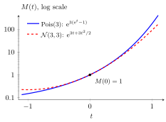
On a logarithmic scale, the MGFs of Poisson(3) and of the normal distribution with mean 3 and variance 3, which touch at t = 0 but separate on either side.

The Poisson and normal laws shown both have mean $3$ and variance $3$ , so their MGFs have the same value and the same first two derivatives at $t=0$ $0$ , where the curves touch. Away from $0$ they separate: at $t=1$ the $\operatorname{Pois}(3)$ MGF is $\mathrm{e}^{3(\mathrm{e}-1)}\approx173$ and the $\mathcal{N}(3,3)$ MGF is $\mathrm{e}^{4.5}\approx90$ $90$ . Already the third derivatives at $0$ differ, since $\mathbb{E}[X^3]=57$ for the Poisson law and $54$ for the normal law. Agreement of a few derivatives is not enough; the whole function near $0$ must match.

Both parts of the hypothesis matter. Equality at $t=0$ alone is automatic, since every MGF equals $1$ there. The MGFs must also be finite near zero: for the lognormal distribution the MGF is infinite for every $t>0$ $0$ , and then the theorem gives no information.

The theorem concerns distributions only. Equal MGFs do not make the variables equal as outcomes, nor independent: for $X\sim\mathcal{N}(0,1)$ $N (0, 1)$ , the variable $-X$ has the same MGF $\mathrm{e}^{t^2/2}$ , yet $-X\neq X$ whenever $X\neq0$ $0$ .

Key Results¶

Equality on an open interval containing zero is sufficient; equality only at zero is not.
Matching a computed MGF to a known MGF identifies the distribution under the same finiteness condition.

Examples¶

If $M_X(t)=\exp(3(\mathrm{e}^t-1))$ near zero, then $X\sim\operatorname{Pois}(3)$ $Pois (3)$ .
If $M_X(t)=\mathrm{e}^{2t+9t^2/2}$ near zero, then $X\sim\mathcal{N}(2,9)$ $N (2, 9)$ , with variance $9$ .

Prerequisites¶

Moment Generating Function

Sources¶

Nicky van Foreest · Probability Distributions · Week 1

Aliases: MGF uniqueness theorem, uniqueness of the MGF

Last updated: 20 October 2026 03:02