Lognormal Distribution¶

Definition¶

Let $Y$ be normally distributed with mean $\mu$ and variance $\sigma^2$ . The random variable $X=\mathrm{e}^Y$ has a lognormal distribution with parameters $\mu$ and $\sigma^2$ .

Interpretation¶

A lognormal variable is a positive quantity whose logarithm is normal. It suits quantities that change by percentages rather than by fixed amounts, such as prices or incomes: a multiplicative change in $X$ is an additive change in $\ln X$ .

A right-skewed lognormal density with three vertical lines for the mode, about 0.78, the median 1 and the mean, about 1.13, from left to right.

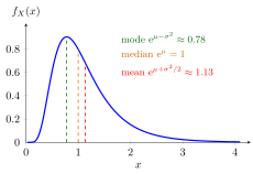
The figure shows $X=\mathrm{e}^Y$ with $Y\sim\mathcal{N}(0,0.5^2)$ $N (0, 0. 5^{2})$ . All probability lies on $x>0$ $0$ , and the density has a long right tail. The three dashed lines are, from left to right, the mode $\mathrm{e}^{\mu-\sigma^2}\approx0.78$ $0.78$ , the median $\mathrm{e}^{\mu}=1$ and the mean $\mathrm{e}^{\mu+\sigma^2/2}\approx1.13$ $1.13$ , the usual order for a right-skewed density.

Change $\mu$ and $\sigma$ of the underlying normal $Y$ : the density of $X=\mathrm e^Y$ is skewed to the right, and more so as $\sigma$ grows.

Because the exponential function is strictly increasing, $X\le x$ if and only if $Y\le\ln x$ $ln x$ . Hence, for $x>0$ $0$ ,

F_X(x)=\Phi\left(\frac{\ln x-\mu}{\sigma}\right),

and every lognormal probability is a standard normal probability. Quantiles carry over in the same way, which is why the median of $X$ is $\mathrm{e}^{\mu}$ : the median of $Y$ is $\mu$ . The density itself follows from the transformation formula with $g(y)=\mathrm{e}^y$ $e^{y}$ .

The mean does not carry over like this: $\mathbb{E}[X]=\mathrm{e}^{\mu+\sigma^2/2}$ is larger than $\mathrm{e}^{\mathbb{E}[Y]}=\mathrm{e}^{\mu}$ $e^{μ}$ . The parameters $\mu$ and $\sigma^2$ are the mean and variance of $\ln X$ , not of $X$ .

Key Results¶

A lognormal random variable is always positive.
If $X$ is lognormal, then $\log X$ is normal.
Lognormal models often arise from products of many positive random factors.

Examples¶

Household income is often modelled with a lognormal-type distribution.
Multiplicative investment growth can lead to lognormal returns over time.
Repair times that are positive and right-skewed may be approximated by a lognormal model.

Prerequisites¶

Sources¶

Probability Theory for EOR · Week 6

Aliases: log-normal distribution Keywords: exponentiated normal distribution Symbols: mu, phi, sigma

Last updated: 20 October 2026 03:02