Exponential Distribution¶

Definition¶

Let $\lambda>0$ $0$ . A continuous random variable $X$ has an exponential distribution with rate $\lambda$ , written $X\sim\operatorname{Exp}(\lambda)$ $Exp (λ)$ , if its density is

\begin{aligned} f_X(x)&=\lambda \mathrm{e}^{-\lambda x}\quad(x>0),\\ f_X(x)&=0\quad(x\le0). \end{aligned}

The parameter $\lambda$ is a rate, not a scale: $\mathbb{E}X=1/\lambda$ and $\operatorname{Var}(X)=1/\lambda^2$ $1/ λ^{2}$ . Assigning any nonnegative density value at $x=0$ does not change the distribution.

Interpretation¶

The exponential distribution is the standard model for a waiting time without memory: the time until the next arrival, failure or decay, when having waited for a while does not change the outlook for the remaining wait. Its rate $\lambda$ is the inverse of the mean waiting time.

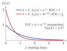
Two exponential densities, with rate 1 and rate 2; the curve with rate 2 starts higher and falls faster.

Both densities start at height $\lambda$ at $x=0$ and then decrease. The red curve with $\lambda=2$ starts twice as high and falls faster, so its probability is concentrated on short waits and its mean is $\tfrac{1}{2}$ instead of $1$ . Each density is highest at $0$ , so an interval of a given length near $0$ carries more probability than one further out, even though the mean is $1/\lambda$ .

Raise the rate $\lambda$ : the density starts higher and falls faster, and the mean waiting time $1/\lambda$ shrinks.

The tail probability $\mathbb{P}(X>x)=\mathrm{e}^{-\lambda x}$ is the formula to remember (later courses call it the survivor function). Each extra unit of time multiplies it by the same factor $\mathrm{e}^{-\lambda}$ , which is the memoryless property: having waited $s$ , the remaining wait is again $\operatorname{Exp}(\lambda)$ . The geometric distribution is the discrete counterpart, with $\mathbb{P}(G\ge n)=(1-p)^n$ $p)^{n}$ .

The parameter is a rate, not a mean: $\operatorname{Exp}(2)$ has mean $\tfrac{1}{2}$ , not $2$ . Some books parametrize by the mean instead, so the convention has to be checked before using a formula.

In a Poisson process with rate $\lambda$ the times between arrivals are independent $\operatorname{Exp}(\lambda)$ variables; the minimum of independent exponentials is exponential with the rates added; and the half-life $\ln 2/\lambda$ is its median.

Key Results¶

For $x\ge0$ $0$ , $F_X(x)=1-\mathrm{e}^{-\lambda x}$ and $\mathbb{P}(X>x)=\mathrm{e}^{-\lambda x}$ $e^{- λ x}$ .
$\mathbb{E}X=1/\lambda$ and $\operatorname{Var}(X)=1/\lambda^2$ $1/ λ^{2}$ .

Examples¶

For $\lambda=2$ $2$ , the mean is $1/2$ and $\mathbb{P}(X>1)=\mathrm{e}^{-2}$ $e^{- 2}$ .
At rate $\lambda=1/5$ per minute, the mean wait is $5$ minutes and $\mathbb{P}(X\le5)=1-\mathrm{e}^{-1}$ $e^{- 1}$ .

Further Properties¶

In a homogeneous Poisson process with rate $\lambda$ , interarrival times are independent $\operatorname{Exp}(\lambda)$ variables.

Prerequisites¶

Sources¶

Probability Theory for EOR · Week 6
Nicky van Foreest · Probability Distributions · Week 2

Aliases: Expo(lambda), exponential random variable, negative exponential distribution, Exp(lambda) Keywords: exponential waiting time, Exponential Symbols: lambda

Last updated: 20 October 2026 03:02