Transformation of a Continuous Random Variable¶

Theorem¶

Let $X$ have a density on an interval $I$. Suppose $g\colon I\to J$ is a continuously differentiable bijection with $g'(x)\ne0$ on $I$. For the transformed variable $Y=g(X)$ and $y\in J$$J$,

and the density is zero outside $J$. Density values at endpoints do not affect probabilities. The absolute derivative accounts for interval stretching; non-strict monotonicity alone is insufficient for this formula. For transformations with suitable monotone branches, add the contributions from each inverse branch.

Interpretation¶

A monotone transformation changes a density by stretching or compressing intervals. The absolute inverse derivative compensates for this change of scale.

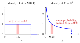
In the illustrated example, $f_Y(y)=f_X\big(g^{-1}(y)\big)\Big|\dfrac{\mathrm{d}}{\mathrm{d}y}g^{-1}(y)\Big|=1\cdot\dfrac{1}{2\sqrt y}$ on $(0,1]$ for $g(x)=x^2$$x^2$. The derivative factor rescales the density so that each strip keeps its probability and the total area stays $1$.

A continuous random variable assigns probabilities through a probability density function. Integration by substitution type 1 transfers those probabilities through the change of variable. Derivative and differentiability describes local interval stretching, and the inverse function theorem gives the reciprocal derivative of the inverse when the derivative of $g$ is nonzero.

Key Results¶

• If $Y=a+bX$ with $b\ne0$$0$, then $f_Y(y)=f_X((y-a)/b)/|b|$$a)/b)/|b|$.
• For a suitable finite collection of monotone branches, sum $f_X(x)/|g'(x)|$ over the preimages $g(x)=y$$y$.

Examples¶

• If $X\sim\operatorname{Unif}(0,1)$ and $Y=2X+1$$1$, then $f_Y(y)=1/2$ on $(1,3)$.
• If $X\sim\operatorname{Unif}(0,1)$ and $Y=X^2$$X^2$, then $f_Y(y)=1/(2\sqrt y)$ on $(0,1)$.

Further Properties¶

The transformed density integrates to one. In higher-dimensional transformations, a Jacobian determinant provides the corresponding volume adjustment.

Prerequisites¶

• Continuous Random Variable
• Probability Density Function
• Derivative and Differentiability
• Inverse Function Theorem
• Integration by Substitution Type 1

Related Concepts¶

• Function of a Random Variable
• Determinant
• Composition of Functions
• LOTUS
• Convolution of Independent Random Variables
• Universality of the Uniform and CDF Realizability

Sources¶

• Probability Theory for EOR · Week 5
• Nicky van Foreest · Probability Distributions · Week 3

Aliases: density transformation formula Keywords: change of variables, transformed random variable, distribution transformation, Change of Variables in One Dimension Symbols: element of, square root

Last updated: 17 October 2026 21:53