Quantile Function¶

Definition¶

For a CDF $F$ and $0<u<1$ $1$ , its generalized inverse is

F^{-1}(u)=\inf\{x\in\mathbb{R}\colon F(x)\ge u\}.

It need not be an ordinary inverse: $F$ can have flat portions or jumps. Endpoint values at $u=0,1$ are irrelevant when using a continuous uniform input.

Interpretation¶

The quantile function answers the reverse question of the CDF. The CDF asks for the probability of being at most $x$ ; the quantile function asks for the threshold below which a fraction $u$ of the probability lies. It converts a probability level into a value of $X$ .

An S-shaped CDF read backwards: from the probability u = 0.8 on the vertical axis across to the curve and down to the quantile Q(u) on the horizontal axis.

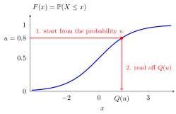
To read the figure, start at the level $u=0.8$ on the vertical axis, move right until the curve is reached, then move down to the horizontal axis: the value found there is $Q(0.8)$ , about $1.39$ for this CDF. Here $Q$ is the $F^{-1}$ of the Definition; when $F$ is continuous and strictly increasing, as here, it is the ordinary inverse, and $F(Q(u))=u$ $u$ .

Pick a level $u$ and read the CDF backwards. At a jump many levels share one quantile, and where $F$ is flat the infimum picks the left end.

The infimum handles the two cases in which no ordinary inverse exists. If $F$ jumps over the level $u$ , no $x$ has $F(x)=u$ $u$ , and $F^{-1}(u)$ is the location of the jump. If $F$ equals $u$ on a whole interval, many $x$ have $F(x)=u$ $u$ , and the infimum picks the left end. In the $\operatorname{Bern}(0.3)$ example the two cases together give $F^{-1}(u)=0$ for $0<u\le0.7$ $0.7$ . By right-continuity of $F$ , $F^{-1}(u)$ is the smallest $x$ with $F(x)\ge u$ $u$ .

Special levels have their own names: $F^{-1}(\tfrac{1}{2})$ is a median, and $F^{-1}(0.25)$ and $F^{-1}(0.75)$ are the lower and upper quartiles. Feeding a uniform input into $F^{-1}$ produces a variable with CDF $F$ , the universality of the uniform used to simulate a distribution.

Despite the notation, $F^{-1}$ is an inverse function, not the reciprocal $1/F$ .

Key Results¶

For $0<u<1$ $1$ , $F^{-1}(u)\le x$ if and only if $u\le F(x)$ $F (x)$ .
Consequently, if $U\sim\operatorname{Unif}(0,1)$ $Unif (0, 1)$ , $\mathbb{P}(F^{-1}(U)\le x)=F(x)$ $F (x)$ .

Examples¶

For $\operatorname{Exp}(2)$ , $F^{-1}(u)=-\log(1-u)/2$ $u) /2$ .
For $\operatorname{Bern}(0.3)$ , $F^{-1}(u)=0$ for $0<u\le0.7$ and $1$ for $0.7<u<1$ $1$ .

Further Properties¶

The median is a quantile at probability level $1/2$ . Other probability levels define percentiles. The generalized inverse is useful even when an ordinary inverse does not exist.

Prerequisites¶

Cumulative Distribution Function

Sources¶

Probability Theory for EOR · Week 5
Nicky van Foreest · Probability Distributions · Week 2

Aliases: Quantile Function (Generalized Inverse CDF), generalized inverse CDF, inverse distribution function, inverse CDF, percent-point function, percentile function, distributional inverse, Quantile Function Symbols: element of, real numbers

Last updated: 20 October 2026 03:02