Conditional Probability
Definition
Let be events with . The conditional probability of given is
This definition restricts and renormalizes the probability model to . It is not defined when , because the quotient would divide by zero.
Interpretation
Conditioning asks how likely is once we know that has happened. The outcomes outside are discarded, and the probabilities of the outcomes in are rescaled so that they sum to one again.
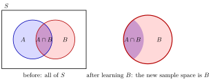
Before conditioning, the whole rectangle counts. After learning , only the disc remains as the new sample space, and of only the part is still possible. is the share of the probability of that lies in .
Knowing that happened keeps only the outlined region. is the share of that region taken up by .
Each part of the formula has a role. The numerator is , not , because outcomes of outside have been ruled out. Dividing by makes the new probabilities add up to one, and it requires : the formula does not define conditioning on an event of probability zero. With equally likely outcomes, as in naive probability, the formula becomes counting inside : . For two fair dice, , but among the six pairs with sum exactly two contain a six, so .
A common slip is to swap the roles of and : in general , and Bayes' rule converts one into the other; confusing them is the prosecutor's fallacy. When , learning changes nothing, which is the idea of independent events. The law of total probability builds back from the conditional probabilities given the cases of a partition.
Key Results
- .
- For fixed of positive probability, is a probability measure.
Examples
- For a fair die, .
- If and , then .
Prerequisites
Related Concepts
Sources
- Probability Theory for EOR · Week 2
- Nicky van Foreest · Probability Distributions · Refresher
Aliases: conditional probability of A given B Keywords: updated probability Symbols: intersection
Last updated: 20 October 2026 03:02
Conditional ProbabilityBayes RuleConditional Expectation Given an EventConditional IndependenceLaw of Total ProbabilityMemoryless PropertyMixture DistributionProsecutor's FallacyBayes and Total Probability: Four FormsConditional Density Given an EventConditional Probability Mass FunctionTotal Probability with Extra ConditioningActuarial Survival and Death ProbabilitiesFuture LifetimeCommon PriorSystem of BeliefsBonus-Malus Transition MatrixOrdinary DeductibleMarkov ChainProbability FunctionUnion and Intersection of EventsIntersection of SetsIndependent EventsAxioms of ProbabilityMultiplication Rule for Counting