Normal Demand Distribution¶

Definition¶

In the course's normal demand approximation, $D\sim \mathcal{N}(\mu,\sigma^2)$ with standard deviation $\sigma>0$ $0$ . If $\Phi$ is the standard normal CDF, then

\begin{gathered} F(y)=\Phi\!\left(\frac{y-\mu}{\sigma}\right),\\ y^*=\max\!\left\{0,\mu+\sigma\Phi^{-1}(\beta)\right\}. \end{gathered}

Interpretation¶

Normal demand is described by two numbers: the mean $\mu$ , the typical demand level, and the standard deviation $\sigma$ , the typical size of deviations from it. The optimal order starts from $\mu$ and adds a safety amount $\sigma\Phi^{-1}(\beta)$ , which depends on the costs only through the critical ratio.

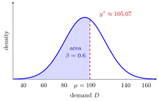
A normal demand density with mean 100 and the area up to about 105.07 shaded, equal to the critical ratio 0.6, which gives the optimal order quantity.

The bell curve is the demand density, centred at $\mu=100$ with $\sigma=20$ $20$ ; areas under it are probabilities. The shaded area to the left of $y^*\approx105.07$ equals $\beta=0.6$ $0.6$ . Since $\Phi^{-1}(0.6)\approx0.2533$ $0.2533$ , the order lies about a quarter of a standard deviation above the mean: $100+20\cdot0.2533\approx105.07$ $105.07$ .

Standardizing turns the continuous newsvendor rule $F(y)=\beta$ into $(y-\mu)/\sigma=\Phi^{-1}(\beta)$ $Φ^{- 1} (β)$ , a single look-up in the standard normal table, and the quantile is then rescaled. If $\beta>\tfrac{1}{2}$ $\frac{1}{2}$ , the order lies above the mean; if $\beta<\tfrac{1}{2}$ $\frac{1}{2}$ , below it; and $\beta=\tfrac{1}{2}$ gives $y^*=\mu$ $μ$ . More uncertainty, a larger $\sigma$ , moves the order further from the mean in the same direction.

A common slip is to use the variance $\sigma^2$ instead of $\sigma$ : with $\sigma^2=400$ the meal example would give an order of about $201$ instead of $105$ . The normal model also gives some probability to negative demand; this hardly matters when $\mu$ is several standard deviations above $0$ , and if the formula gives a negative quantity the order is $0$ .

Key Results¶

Use the standard deviation $\sigma$ , not the variance $\sigma^2$ , in the quantile formula.
The order quantity must satisfy $y\ge0$ $0$ . Use the normal quantile when it is nonnegative; otherwise the constrained optimum is $y^*=0$ $0$ .
The untruncated normal distribution allows negative values; the course examples retain that approximation.
The normal table gives rounded quantiles.

Examples¶

The shaded area in the figure is $\mathbb{P}(D\le y^*)=0.6$ $0.6$ . Table values $\Phi(0.25)=0.5987$ and $\Phi(0.26)=0.6026$ bracket the standardized quantile between 0.25 and 0.26.

Meal demand with $\mu=100$ $100$ , $\sigma=20$ and $\beta=0.6$ gives about 105.07.
For apples, $\beta=1.8/2.2\approx0.8182$ and the source table approximation $z\approx0.91$ gives 82.75 kilograms.

Prerequisites¶

Continuous Newsvendor Rule
Normal distribution

Sources¶

OR Modelling · Week 6

Aliases: normal demand approximation Symbols: beta, mu, phi, sigma

Last updated: 20 October 2026 03:02