Graphical Method¶

Definition¶

The graphical method solves a two-variable LP by drawing each constraint boundary, identifying the common feasible region, drawing a constant-objective line, and moving that line in the direction of improvement until the best feasible contact is reached. Intersecting the relevant boundary equations gives exact coordinates.

Interpretation¶

The method makes feasibility and optimality visible. It also reveals whether the best value is attained at one point or along a segment.

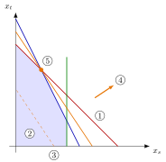
The feasible pentagon with numbered steps: boundary lines, the shaded region, a dashed objective line, the direction to slide it, and the last point of contact at the optimum.

The numbered markers illustrate the method for the objective $z=3x_s+2x_t$ $2 x_{t}$ :

Draw the boundaries $2x_s+x_t=100$ $100$ , $x_s+x_t=80$ and $x_s=40$ $40$ .
Shade their common feasible region, including the restrictions $x_s,x_t\ge0$ $0$ .
Draw a constant-objective line, such as the dashed line $3x_s+2x_t=90$ $90$ .
Move the line in the improving direction $(3,2)$ while it still touches the feasible region.
The last contact is the optimum, here the corner $(20,60)$ .

Key Results¶

Determine the allowed side of each boundary from the inequality; do not assume it is always below the line.
Check the direction of improvement from the objective, especially with negative coefficients.
Also allow for an empty feasible region or an objective that can improve without bound.

Examples¶

Maximizing $x_1+2x_2$ with $x_1\le4$ $4$ , $x_2\le5$ $5$ , $2x_1+x_2\le9$ gives $(2,5)$ .
For $z=2x_1-3x_2$ $3 x_{2}$ , increasing $z$ moves its objective line downward.

Prerequisites¶

Sources¶

OR Modelling · Week 1

Aliases: graphical solution method, graphical solution procedure

Last updated: 20 October 2026 03:02