Multiple Optimal Solutions¶

Definition¶

An optimization problem has multiple optimal solutions if distinct feasible decision vectors attain the same optimal objective value. In an LP, every convex combination of two optimal solutions is also optimal.

Interpretation¶

Different decisions can be equally good under the stated objective. In a two-variable LP, this often appears as an objective line coinciding with a feasible boundary segment.

The figure and the interactive example both use the feasible region of the Giapetto production model: $x_s$ wooden soldiers and $x_t$ trains, with finishing $2x_s+x_t\le100$ $100$ , carpentry $x_s+x_t\le80$ and soldier demand $x_s\le40$ $40$ . Only the objective is changed, so that it becomes parallel to one edge.

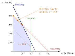
The Giapetto feasible pentagon with its finishing, carpentry and demand lines, the dashed objective line z = 100, and the whole carpentry edge from (0, 80) to (20, 60) marked as optimal with value 160.

With $z=2x_s+2x_t$ $2 x_{t}$ , every objective line $x_s+x_t=z/2$ is parallel to the carpentry edge. Pushing the dashed line $z=100$ outwards, it leaves the region along the whole edge from $(0,80)$ to $(20,60)$ , where $z=160$ $160$ .

Key Results¶

A zero objective-row coefficient for a nonbasic variable in an optimal simplex tableau suggests an alternative optimum.
A positive feasible movement in that direction produces a distinct optimum; a zero-length degenerate pivot alone does not establish a different decision vector.
Additional requirements can select one point from an optimal segment.

Examples¶

For the illustrated objective $2x_s+2x_t$ $2 x_{t}$ , the feasible part of $x_s+x_t=80$ between $(0,80)$ and $(20,60)$ is optimal. It includes $(10,70)$ ; every point on the segment has value 160.
For the interactive objective $4x_s+2x_t$ $2 x_{t}$ , the five corners $(0,0)$ , $(40,0)$ , $(40,20)$ , $(20,60)$ , $(0,80)$ give $0$ , $160$ , $200$ , $200$ , $160$ , so the edge from $(40,20)$ to $(20,60)$ is optimal with value 200.
Adding the requirement $x_s=30$ to that problem selects the single point $(30,40)$ of the optimal edge: $2\cdot30+40=100$ and $4\cdot30+2\cdot40=200$ $200$ .
With the original Giapetto profit $3x_s+2x_t$ $2 x_{t}$ , the corner values are $0,120,160,180,160$ , so the optimum $(20,60)$ is unique.
The Week 3 course materials (data not reproduced here) give another LP in which $(5,0)$ and $(3,4)$ both attain $4x_1+2x_2=20$ $20$ ; in practice exercise 3 of Week 3, imposing $x_1=1$ selects $(1,9/2)$ from the optimal segment.

Prerequisites¶

Sources¶

OR Modelling · Week 1

Aliases: alternative optima, alternative optimal solutions, multiple optima, alternate optima

Last updated: 20 October 2026 03:02