Newsvendor Model¶

Definition¶

The newsvendor model chooses a single order quantity $y\ge0$ before observing random demand $D$. With unit purchase cost $c$, selling price $p>c$$c$, and salvage value $s<c$$c$, define overage cost $h=c-s$ and underage cost $b=p-c$$c$. Minimize

where $u^+=\max\{u,0\}$ and the expectations are finite. Sales equal $\min\{y,D\}$.

Interpretation¶

The newsvendor model chooses one stock level before an uncertain demand is seen, for a product that cannot be sold later at full price. Too much stock leaves units that are sold off at the salvage value, costing $h=c-s$ each; too little misses sales that would have earned $b=p-c$ each.

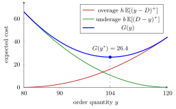
In the meal example, demand lies between $80$ and $120$ with all values equally likely, and $h=2.2$$2.2$, $b=3.3$$3.3$. Raising $y$ increases the expected cost of leftovers (red) and decreases the expected cost of missed sales (green). The sum $G(y)$ is lowest at $y^*=104$$104$, with value $26.4$.

The optimum can be found by asking whether one more unit is worth stocking: it is left over if demand is at most $y$, costing $h$, and sells if demand is above $y$, saving $b$. Adding it pays off as long as $b$ times the chance that demand exceeds $y$ is larger than $h$ times the chance that it does not. In the example, the chance that demand is at most $y$ is $(y-80)/40$$80)/40$, and the two sides balance when this chance equals $b/(b+h)=0.6$$0.6$, at $y=104$$104$. The positive part $(y-D)^+$ counts leftovers and $(D-y)^+$ missed sales, so each gets its own unit cost.

Unlike the EOQ models, there is a single period and no setup cost, and unmet demand is lost rather than backlogged. The balance point $b/(b+h)$ is developed further as the critical ratio.

Key Results¶

• Salvage value can be zero or negative.
• $G(y)$ is convex; an optimum occurs where increasing stock stops reducing expected cost.
• $G(y)$ measures overage and underage loss, not gross purchasing expenditure.
• The model is introduced in the week 5 overview and developed in week 6.

Examples¶

The illustrated meal-demand example is uniform on $[80,120]$ with critical ratio $\beta=0.6$$0.6$. Its optimal stock is $y^*=104$$104$, for which $F(104)=0.6$$0.6$.

• A newsvendor chooses newspaper stock before daily demand is known.
• A shop chooses seasonal dress inventory; a canteen prepares meals before evening demand.

Prerequisites¶

• Inventory Policy
• Positive Part
• Random variables and expectation

Related Concepts¶

• Overage Cost
• Underage Cost
• Critical Ratio

Sources¶

• OR Modelling · Week 5

Aliases: newsboy problem, newsvendor problem, newsboy model, news vendor problem Symbols: beta

Last updated: 20 October 2026 03:02