Unbounded Linear Program¶

Definition¶

A maximization LP has an unbounded objective if feasible solutions attain objective values greater than any prescribed finite bound. For minimization, feasible values can be arbitrarily negative. In a feasible maximization tableau, an improving entering column with no strictly positive constraint coefficient certifies unboundedness.

Interpretation¶

An unbounded linear program has feasible solutions but no optimal one: whatever objective value is reached, another feasible solution does better. In an applied model this is a signal to check whether a restriction, such as a limit on demand or capacity, is missing.

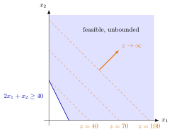
An unbounded shaded region above the line 2x1 + x2 = 40 with objective lines for z = 40, 70 and 100 and an arrow showing that z can grow without limit.

The shaded region, given by $2x_1+x_2\ge40$ and $x_1,x_2\ge0$ $0$ , is open towards the upper right. The dashed objective lines $x_1+x_2=40$ $40$ , $70$ and $100$ all meet the region, and moving the line further out never leaves it, so $z=x_1+x_2$ can be made as large as desired.

The simplex method detects this in the tableau. The minimum-ratio test normally limits how far an improving entering variable $x_k$ can increase before a basic variable reaches zero. A coefficient $a_{ik}\le0$ in the entering column means that the basic variable of row $i$ does not decrease as $x_k$ grows. If the whole column has no positive entry, $x_k$ can grow without limit while all basic variables stay nonnegative, and $z$ grows with it.

Unboundedness is a property of the objective on the region, not of the region alone. An unbounded feasible region can still have a finite optimum: minimizing $x_1+x_2$ over the region in the figure gives the optimum $20$ at $(20,0)$ . An unbounded LP should also not be confused with an infeasible one, which has no feasible solution at all.

Key Results¶

An unbounded feasible region can still have a finite optimum for a particular objective.
The simplex certificate requires an improving objective coefficient and an unrestricted feasible increase together.
Do not confuse unboundedness with infeasibility.

Examples¶

The figure maximizes $x_1+x_2$ subject to $2x_1+x_2\ge40$ and $\boldsymbol{x}\ge0$ $0$ . Taking $x_1=t$ $t$ , $x_2=0$ for $t\ge20$ gives feasible values growing without bound. In an applied model, such a result can indicate a missing restriction rather than automatically proving a modelling error.

In week 2 practice 1(c), $x_1=0$ $0$ , $x_2=t\ge0$ satisfies $3x_1-2x_2\le8$ and gives $z=t$ $t$ .
In the week 3 example, $x_1=x_2=t$ is feasible and yields $2x_1+x_2=3t$ $3 t$ .

Prerequisites¶

Sources¶

OR Modelling · Week 2

Aliases: unbounded objective, unbounded LP Keywords: Unbounded objective value

Last updated: 20 October 2026 03:02