Linear Programming¶

Definition¶

A linear program (LP) maximizes or minimizes a linear objective function subject to linear equality and/or inequality constraints. Its decision variables are continuous; if additional integer restrictions are imposed, the model becomes an integer linear program rather than an LP. For example,

\begin{gathered} \max z=\sum_{j=1}^n c_jx_j,\\ \sum_{j=1}^n a_{ij}x_j\le b_i\ (i=1,\ldots,m),\\ x_j\ge0. \end{gathered}

Other inequality directions and equalities are also allowed in an LP.

Interpretation¶

A linear program optimizes a linear objective over the decisions allowed by linear constraints. "Linear" means that each variable enters only multiplied by a constant, and the terms are added, as in $3x_s+2x_t$ $2 x_{t}$ . This simple form is what makes large planning models tractable.

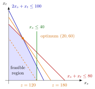
The feasible pentagon of a production problem with two objective lines, z = 120 and z = 180, the second touching the region at the optimal corner (20, 60).

The figure shows what linearity looks like in two variables. Every constraint boundary is a straight line, so the feasible region is a polygon with straight edges, and every set of points with equal objective value is a straight line; the lines $z=120$ and $z=180$ are parallel. The best value $180$ is reached where the highest objective line still touches the region, at the corner $(20,60)$ .

The definition rules out products such as $x_1x_2$ , powers such as $x_j^2$ and fractions with a variable in the denominator, although some fractions can be multiplied out, as the share constraint of the diet problem shows. Variables are continuous, so $20.5$ soldiers is an allowed value; indivisible decisions need explicit integer restrictions. The definition does not promise an optimum either: the constraints may contradict each other, or the objective may improve without limit.

Two variables can be handled by the graphical method; larger LPs are solved by the simplex method, which moves from corner to corner of the region.

Key Results¶

Products of decision variables and powers such as $x_j^2$ are not linear.
Negative coefficients are allowed.
The graphical method is useful for two variables; simplex handles larger models.

Examples¶

The illustrated Giapetto LP has objective $3x_s+2x_t$ and attains value 180 at $(20,60)$ . Its original quantities are continuous; no integrality restriction is included.

Giapetto maximizes $3x_s+2x_t$ under linear labour and demand limits.
The diet problem minimizes cost under nutrient and composition requirements.

Prerequisites¶

Sources¶

OR Modelling · Week 1

Aliases: LP, linear optimization, linear optimisation Keywords: linear program Symbols: sum

Last updated: 27 October 2026 11:52