Assignment Cost Transformation¶

Proposition¶

In a square one-to-one assignment problem, adding a constant $a_i$ to every cost in row $i$ , or a constant $b_j$ to every cost in column $j$ , preserves the set of optimal assignments. Every complete assignment's cost changes by the same total $\displaystyle \sum_i a_i+\sum_j b_j$ $j \sum b_{j}$ .

Interpretation¶

Every complete assignment uses each row and each column of the cost table exactly once. Adding a constant to a whole row or column therefore adds it exactly once to every complete assignment: all totals shift by the same amount and the ranking is unchanged.

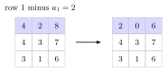
A 3 by 3 cost matrix before and after subtracting 2 from its first row; the highlighted first row is lower by exactly 2, so every complete assignment total also falls by 2.

In the figure only row $1$ changes: its entries $4,2,8$ become $2,0,6$ . Whichever task agent $1$ receives, that one entry is $2$ lower, so every complete assignment costs $2$ less, as the table in the Examples confirms for three of them.

The argument needs every row and every column to be used exactly once, which is why it applies to the square assignment problem. In a rectangular table without dummy entries, some agent stays unused, and changing that agent's row alters only the assignments that use the agent, which can change the optimum. Changing a single entry, or multiplying a row by a factor, can also change which assignment is best.

The transformation is the engine of the Hungarian algorithm. If the subtracted constants keep all entries nonnegative, every complete assignment costs at least the total amount subtracted, and an assignment that uses only zero entries reaches this bound, so it is optimal. The transformed totals only rank the assignments; the cost of the chosen assignment is read from the original table.

Key Results¶

Subtracting row and column minima is a valid transformation.
The Hungarian uncovered-entry adjustment is equivalent to suitable row and column changes.
For a maximum-profit assignment, negate profits and add a constant large enough to make the resulting costs nonnegative.

Examples¶

In the figure, subtracting $a_1=2$ from row 1 lowers each complete assignment cost by 2. More generally, subtracting row amounts $a_i$ and column amounts $b_j$ changes every complete total by $\displaystyle -\sum_i a_i-\sum_j b_j$ $j \sum b_{j}$ .

Assignment pairs	Original total	Transformed total
$(1,1),(2,3),(3,2)$	$4+7+1=12$	$2+7+1=10$
$(1,2),(2,1),(3,3)$	$2+4+6=12$	$0+4+6=10$
$(1,3),(2,2),(3,1)$	$8+3+3=14$	$6+3+3=12$

If row minima are 2, 5, 6, and 4, subtracting them reduces every assignment cost by 17.
Transforming profits $p_{ij}$ into costs $M-p_{ij}$ changes a complete assignment objective to $\displaystyle nM-\sum_i p_{i,\pi(i)}$ $i \sum p_{i, π (i)}$ , where $\pi(i)$ is the column assigned to row $i$ .

Prerequisites¶

Assignment Problem

Sources¶

OR Modelling · Week 5

Symbols: pi, sum

Last updated: 20 October 2026 03:02