Transportation Problem¶

Definition¶

The transportation problem chooses shipments $x_{ij}\ge0$ from plants $i$ to distribution centres $j$ to minimize total transport cost. With unit costs $c_{ij}$ , plant capacities $s_i$ , and required deliveries $d_j$ , a formulation is

\begin{gathered} \min\sum_i\sum_j c_{ij}x_{ij},\\ \sum_jx_{ij}\le s_i\ \text{for every }i,\\ \sum_ix_{ij}=d_j\ \text{for every }j. \end{gathered}

The demand constraints can also be written as $\displaystyle \sum_ix_{ij}\ge d_j$ $d_{j}$ : when every unit cost $c_{ij}$ is positive, an optimal plan never delivers more than required, so both versions have the same optimal solutions.

Interpretation¶

The transportation problem decides how much to send along each route from origins with limited supply to destinations with given demand, so that the total transport cost is as small as possible. Each decision variable $x_{ij}$ is the amount on one route, and every unit on that route costs $c_{ij}$ .

Two plants with supplies 30 and 20 joined to three customers with demands 15, 20 and 15, with the shipments used in the optimal plan labelled by amount and unit cost.

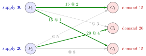
The plants $P_1$ and $P_2$ have supplies $30$ and $20$ , and the customers need $15$ , $20$ and $15$ . The thick edges are the routes in use, labelled amount @ unit cost: $P_1$ sends $15$ to $C_1$ and $15$ to $C_3$ , and $P_2$ sends $20$ to $C_2$ , for a total cost of $125$ . Each customer receives exactly its demand, and the thin routes carry nothing.

Every variable appears in exactly two constraints, the supply constraint $\displaystyle \sum_jx_{ij}\le s_i$ of its origin and the demand constraint of its destination. Supplies use $\le$ because a plant need not use all of its capacity. Adding the demand constraints shows that a feasible plan needs total supply at least total demand, and since every route may be used, this is also enough. When capacity exceeds demand, as in the week 2 data in the Examples, some capacity stays unused.

The model is an ordinary linear program, solvable with the simplex method or Excel Solver. The same bookkeeping returns later in the assignment problem, where every supply and every demand equals $1$ .

Key Results¶

The decision variables are shipment quantities on routes.
Plant capacities are upper bounds rather than mandatory production amounts.
With positive unit costs, allowing deliveries above demand ( $\geq$ $\ge d_j$ instead of $=d_j$ $d_{j}$ ) cannot improve the optimum.

Examples¶

The diagram is a separate balanced illustration with total supply and demand both 50. Its unit costs are $2,3,1$ from $P_1$ to $C_1,C_2,C_3$ and $5,4,8$ from $P_2$ . Green-edge labels mean shipment quantity @ unit cost; their total is $15\cdot2+15\cdot1+20\cdot4=125$ $125$ . The plan is optimal: moving one unit of a customer's delivery from $P_2$ to $P_1$ saves $5-2=3$ for $C_1$ , $4-3=1$ for $C_2$ and $8-1=7$ for $C_3$ , so $P_1$ 's 30 units go to $C_3$ (15) and then $C_1$ (15), and $P_2$ supplies $C_2$ . Because total supply equals total demand, every plant here also ships its full supply. For a feasible transportation LP with integer supplies and demands, an integral optimal shipment plan exists.

Week 2 course data: three plants with capacities 5,000, 6,000 and 2,500 (13,500 in total) serve destinations whose demands total 12,000, so at least 1,500 units of capacity stay unused; with the course's unit costs the optimal cost is 35,000.

Prerequisites¶

Linear Program Formulation

Sources¶

OR Modelling · Week 2

Aliases: transportation model, Hitchcock problem Symbols: sum

Last updated: 20 October 2026 03:02